
Function Convergence and Continuity
Loading the math board and drawing, please wait…
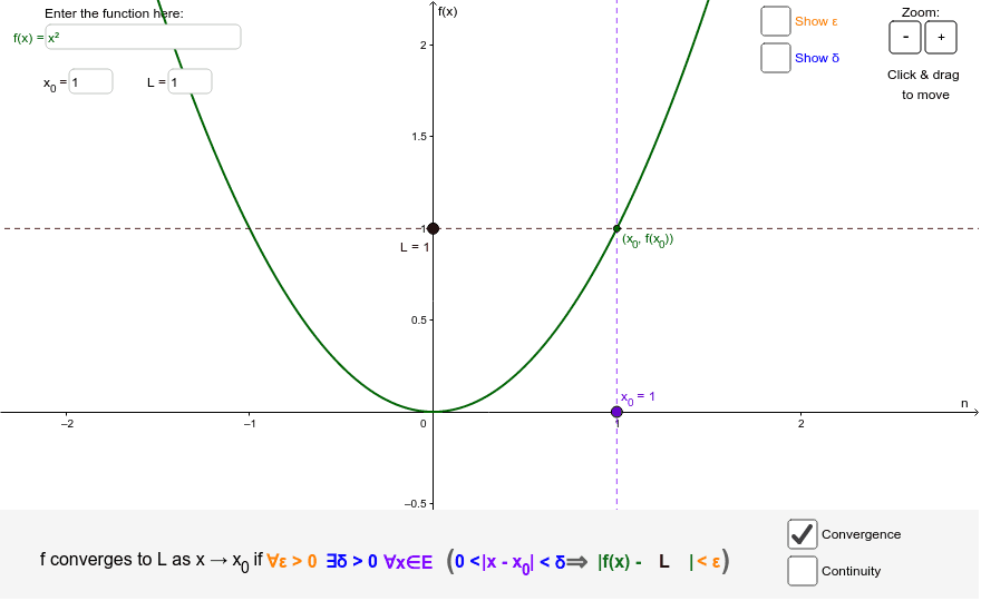
This example demonstrates the ε-δ definition of limit in functions. Key math concepts include limits, continuity, and the ε-δ definition. It uses GeoGebra commands like If, Textfield, Vector, Line, Polygon to dynamically illustrate the changes in ε and δ, explaining the limit definition. Suitable for high school students and beginners in calculus learning the concepts of function limits and continuity.
GeoGebra Commands & Parameters
If(limMode, L1, L2) → LTextfield(f) → fInputVector(LPoint, (x(LPoint), L + epsilon)) → epsilonVectorVector(LPoint, (x(LPoint), L - epsilon)) → epsilonVector2Line(Lpoint1, Lpoint2) → LLineLine(Xpoint1, Xpoint2) → XLineLine(epsTopPoint1, epsTopPoint2) → epsilonTopLineLine(epsBottomPoint1, epsBottomPoint2) → epsilonBottomLinePolygon((viewLeft, L + epsilon), (viewRight, L + epsilon), (viewRight, L - epsilon), (viewLeft, L - epsilon)) → epsilonRegion, a, b, c, eLine(deltaLeftPoint1, deltaLeftPoint2) → deltaLeftLineLine(deltaRightPoint1, deltaRightPoint2) → deltaRightLineVector(XPoint, (X + delta, 0)) → deltaVectorVector(XPoint, (X - delta, 0)) → deltaVector2Polygon((X - delta, viewTop), (X + delta, viewTop), (X + delta, viewBottom), (X - delta, viewBottom)) → deltaRegion, g, h, i, jTextfield(X) → XInputLine((0, L2), (1, L2)) → L2LineTextfield(L1) → LinputPolygon(Corner[1], Corner[2], (0.85 * Corner[2]) + (0.15 * Corner[3]), (0.85 * Corner[1]) + (0.15 * Corner[4])) → poly1, k, l, m, n