
Function Addition Demonstration
Loading the math board and drawing, please wait…
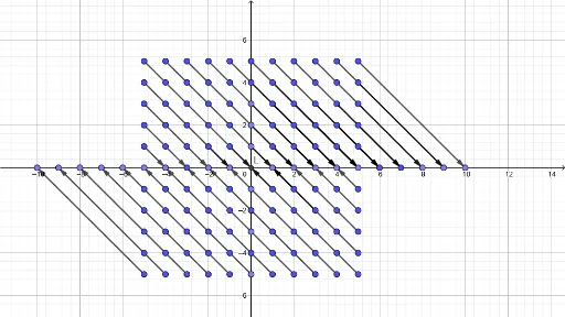
This example demonstrates how to construct a graphical representation of function addition using GeoGebra. It involves core math concepts like functions, vectors, and coordinate geometry. Key GeoGebra commands used include Point, Intersect, and Vector. Suitable for high school mathematics education to understand the geometric meaning of function operations.
GeoGebra Commands & Parameters
Point(yAxis) → APoint(xAxis) → GPoint(xAxis) → HPoint(xAxis) → IPoint(xAxis) → JPoint(xAxis) → KIntersect(xAxis, yAxis) → LPoint(yAxis) → MPoint(yAxis) → SPoint(xAxis) → O_1Point(xAxis) → P_1Point(xAxis) → Q_1Vector(A, K) → uVector(B, J) → vVector(C, I) → wVector(D, H) → aVector(E, G) → bVector(F, M_1) → cVector(M, J) → dVector(N, I) → eVector(O, H) → fVector(P, G) → gVector(Q, M_1) → hVector(R, N_1) → iVector(S, I) → jVector(T, H) → kVector(U, G) → lVector(V, M_1) → mVector(W, N_1) → nVector(Z, O_1) → pVector(A_1, P_1) → qVector(L_1, Q_1) → rVector(K_1, P_1) → sVector(J_1, O_1) → tVector(I_1, N_1) → u_1Vector(H_1, M_1) → v_1Vector(E_1, G) → w_1Vector(F_1, H) → a_1Vector(G_1, G) → b_1Point(yAxis) → R_1Point(yAxis) → F_2Point(yAxis) → R_2Point(xAxis) → Z_2Point(xAxis) → A_3Point(xAxis) → C_3Point(xAxis) → D_3Point(xAxis) → E_3Point(xAxis) → F_3Point(xAxis) → G_3Vector(S_1, L) → c_1Vector(W_2, L) → d_1Vector(T_1, K) → e_1Vector(B_2, K) → f_1Vector(Q_2, K) → g_1Vector(K_2, J) → h_1Vector(Z_1, I) → i_1Vector(W_1, H) → j_1Vector(V_2, Z_2) → k_1Vector(U_2, A_3) → l_1Vector(T_2, B_3) → m_1Vector(S_2, C_3) → n_1Vector(R_2, D_3) → p_1Vector(D_4, E_3) → q_1Point(xAxis) → I_4Point(xAxis) → J_4Vector(E_4, F_3) → r_1Vector(F_4, G_3) → s_1Vector(G_4, I_4) → t_1Vector(H_4, J_4) → u_2Vector(K_4, L) → v_2Vector(K_5, L) → w_2Vector(L_4, Z_2) → a_2Vector(B_5, Z_2) → b_2Vector(A_5, A_3) → c_2Vector(P_4, B_3) → d_2Vector(O_4, C_3) → e_2Vector(J_5, K) → f_2Vector(I_5, J) → g_2Vector(H_5, I) → h_2Vector(G_5, H) → i_2
AI Drawing Prompt Reference
On a coordinate plane, place several points on the y-axis and x-axis, and mark the origin at their intersection. Then draw vectors from each y-axis point to a corresponding x-axis point, and also from each x-axis point to a corresponding y-axis point, creating a set of crossing arrows. These vectors spread on both sides of the axes, with varied directions and lengths, illustrating the geometric idea of adding functions via corresponding point connections. The figure uses the axes as a framework and arrows as key elements.
The prompt above was compiled from the original drawing commands and is for reference only.