Free Fall with Marks and Final Position

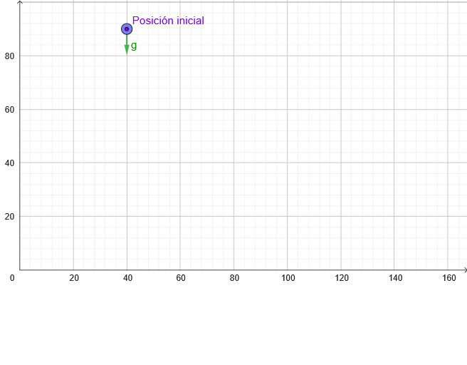
① This GeoGebra example dynamically simulates free fall motion, showing equally spaced time marks along the falling object's path and a final endpoint. ② Core mathematical concepts include uniformly accelerated linear motion, displacement-time relationship, velocity change, sequences (position series), and limits (final position). ③ Construction highlights: uses PointIn and Sequence commands to generate a series of marked points, sliders for time parameters (t0, t1, dt, tt), buttons (anima, reinicia, empieza) and boolean variables (para, verVectores) to control animation and vector display, plus text objects (texto1, texto2) for real-time data. ④ Suitable for high school physics or math classes to teach kinematics, sequences, and limits, as well as to demonstrate dynamic geometry and animation construction in GeoGebra.