
Fraction Division Geometric Demonstration by ericchowyl
Loading the math board and drawing, please wait…
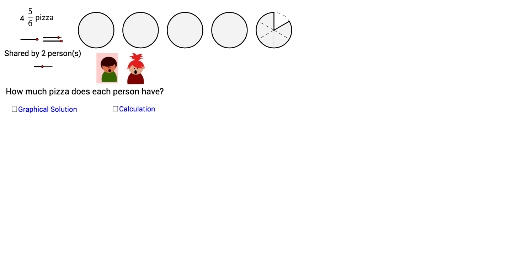
This example demonstrates the concept of fraction division. It involves core mathematical concepts such as fractions and division. Using GeoGebra commands like Segment, Point, Sequence, etc., a geometric model of fraction division is constructed. Suitable for middle school and above students to learn the geometric meaning of fraction division.
GeoGebra Commands & Parameters
Segment(A, (x(A) + 1, y(A))) → l1Point(Segment[(x(A), y(A)), (x(A) + 1, y(A))]) → PSegment(B, (x(B) + 1, y(B))) → l2Point(Segment[(x(B) + 2 / 6, y(B)), (x(B) + 1, y(B))]) → QPoint(Segment[(x(C) + 1 / 6 - 0.005, y(C)), (x(Q) - 1 / 6, y(C))]) → RSegment(C, (x(C) + 1, y(C))) → l3Sequence(Circle[((2.5 * (i - 1)), 0), 1], i, 1, a) → list1Sequence(Sequence[CircleSector[((f * sin((((2 * k) - 1) * θ / 2))) + (2.5 * (m - 1)), (f * cos((((2 * k) - 1) * θ / 2)))), ((f * sin((((2 * k) - 1) * θ / 2))) + sin((k * θ)) + (2.5 * (m - 1)), (f * cos((((2 * k) - 1) * θ / 2))) + cos((k * θ))), ((f * sin((((2 * k) - 1) * θ / 2))) + sin(((k - 1) * θ)) + (2.5 * (m - 1)), (f * cos((((2 * k) - 1) * θ / 2))) + cos(((k - 1) * θ)))], k, 1, b], m, 1, a) → list4Sequence(CircleSector[(((-f) * sin((((2 * k) - 1) * θ / 2))) + (2.5 * a), (f * cos((((2 * k) - 1) * θ / 2)))), (((-f) * sin((((2 * k) - 1) * θ / 2))) - sin(((k - 1) * θ)) + (2.5 * a), (f * cos((((2 * k) - 1) * θ / 2))) + cos(((k - 1) * θ))), (((-f) * sin((((2 * k) - 1) * θ / 2))) - sin((k * θ)) + (2.5 * a), (f * cos((((2 * k) - 1) * θ / 2))) + cos((k * θ)))], k, 1, c) → list5CircleSector(((2.5 * a), 0), ((2.5 * a), 1), ((2.5 * a) - sin((c * θ)), cos((c * θ)))) → s1_1Sequence(Segment[((2.5 * a), 0), ((2.5 * a) - sin((j * θ)), cos((j * θ)))], j, 1, c - 1) → list2Sequence(Segment[((2.5 * a), 0), ((2.5 * a) - sin((j * θ)), cos((j * θ)))], j, c + 1, b - 1) → list3CircleSector(((2.5 * a), 0), ((2.5 * a) - sin((c * θ)), cos((c * θ))), ((2.5 * a), 1)) → s2Segment(D, (x(D) + 1, y(D))) → l4Point(Segment[(x(D) + 1 / 5, y(D)), (x(D) + 1, y(D))]) → SSequence(Sequence[CircleSector[(((-f) * sin((((2 * k) - 1) * θ / 2))) + (2.5 * (m - 1)), (f * cos((((2 * k) - 1) * θ / 2)))), (((-f) * sin((((2 * k) - 1) * θ / 2))) - sin(((k - 1) * θ)) + (2.5 * (m - 1)), (f * cos((((2 * k) - 1) * θ / 2))) + cos(((k - 1) * θ))), (((-f) * sin((((2 * k) - 1) * θ / 2))) - sin(((k - 1) * θ) + θ / d) + (2.5 * (m - 1)), (f * cos((((2 * k) - 1) * θ / 2))) + cos(((k - 1) * θ) + θ / d))], k, 1, b], m, 1, a) → list6Sequence(CircleSector[(((-f) * sin((((2 * k) - 1) * θ / 2))) + (2.5 * a), (f * cos((((2 * k) - 1) * θ / 2)))), (((-f) * sin((((2 * k) - 1) * θ / 2))) - sin(((k - 1) * θ)) + (2.5 * a), (f * cos((((2 * k) - 1) * θ / 2))) + cos(((k - 1) * θ))), (((-f) * sin((((2 * k) - 1) * θ / 2))) - sin(((k - 1) * θ) + θ / d) + (2.5 * a), (f * cos((((2 * k) - 1) * θ / 2))) + cos(((k - 1) * θ) + θ / d))], k, 1, c) → list7Sequence(Sequence[Sequence[Segment[(((-f) * sin((((2 * k) - 1) * θ / 2))) + (2.5 * (m - 1)), (f * cos((((2 * k) - 1) * θ / 2)))), (((-f) * sin((((2 * k) - 1) * θ / 2))) - sin(((k - 1) * θ) + (n * θ / d)) + (2.5 * (m - 1)), (f * cos((((2 * k) - 1) * θ / 2))) + cos(((k - 1) * θ) + (n * θ / d)))], n, 1, d - 1], k, 1, b], m, 1, a) → list8Sequence(Sequence[Segment[(((-f) * sin((((2 * k) - 1) * θ / 2))) + (2.5 * a), (f * cos((((2 * k) - 1) * θ / 2)))), (((-f) * sin((((2 * k) - 1) * θ / 2))) - sin(((k - 1) * θ) + (n * θ / d)) + (2.5 * a), (f * cos((((2 * k) - 1) * θ / 2))) + cos(((k - 1) * θ) + (n * θ / d)))], n, 1, d - 1], k, 1, c) → list9Polygon((0.016528925619834656, -3), (1.2165289256198346, -3), (1.2165289256198346, -1.3), (0.016528925619834656, -1.3)) → poly1, e, g, h, iGCD((a * b) + c - ((floor(((a * b) + c) / ((b * d))) * b) * d), (b * d)) → kSegment(A, P) → jSegment(C, R) → lSegment(B, Q) → mSegment(D, S) → n
AI Drawing Prompt Reference
Create a geometric model to demonstrate the concept of fraction division. Start by drawing two line segments AB and CD, then mark points P on AB, Q and R on CD. Draw a series of circles and arcs, including circles centered on the x-axis and arcs around the origin. Finally, connect points A and P, C and R, B and Q, and D and S to form the geometric model.
The prompt above was compiled from the original drawing commands and is for reference only.