
Fraction Division 4: 1 ÷ a/b (Quotitive) by Mario Villani
Loading the math board and drawing, please wait…
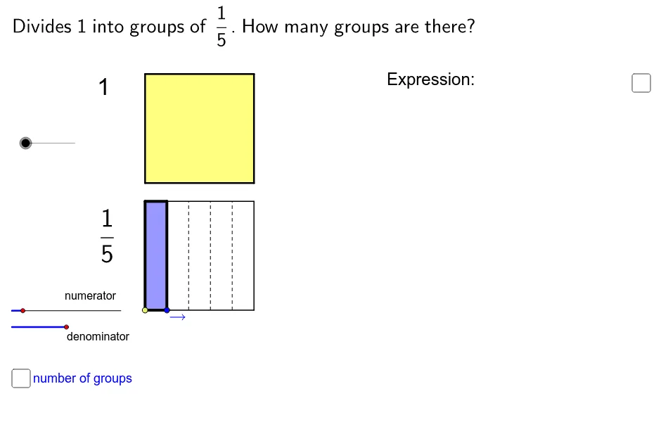
This example demonstrates the graphical interpretation of 1 ÷ a/b = b/a and visually illustrates [i]x[/i] ÷ a/b = [i]x[/i] × b/a in the context of quotitive (measurement) division. Key math concepts include fraction division, quotitive division, fraction multiplication, and proportional relationships. It is constructed using GeoGebra commands like Point, Min, Max, Segment, Polygon, Sequence, If, involving objects such as a, b, gcd, A, s, f_1, etc. Suitable for middle school and above mathematics education to enhance understanding of fraction division concepts.
GeoGebra Commands & Parameters
Point(Segment[(x(E) + 0.1, y(E)), (x(E) + 1, y(E))]) → GPoint(Segment[(x(D) + 0.1, y(D)), (x(D) + 0.5, y(D))]) → FMin(round((x(G) - x(E)) / 0.1), 2 * a') → b'Max(Sequence[If[(Mod[a * a', i] ≤ 0) ∧ (Mod[b', i] ≤ 0), i, 1], i, 1, Min[a * a', b']]) → gcdSegment((0, 1), (x(A), y(A))) → f_1Point(f_1) → BSegment(A, (x(A) + a, y(A))) → lSegment((x(A), y(A) + w), (x(A) + a, y(A) + w)) → mSegment(A, (x(A), y(A) + w)) → nSegment((x(A) + 9, y(A)), (x(A) + 9, y(A) + w)) → pSegment((x(A) + 8, y(A)), (x(A) + 8, y(A) + w)) → qSegment((x(A) + 7, y(A)), (x(A) + 7, y(A) + w)) → rSegment((x(A) + 6, y(A)), (x(A) + 6, y(A) + w)) → tSegment((x(A) + 5, y(A)), (x(A) + 5, y(A) + w)) → a_1Segment((x(A) + 4, y(A)), (x(A) + 4, y(A) + w)) → b_1Segment((x(A) + 3, y(A)), (x(A) + 3, y(A) + w)) → c_1Segment((x(A) + 2, y(A)), (x(A) + 2, y(A) + w)) → d_1Segment((x(A) + 10, y(A)), (x(A) + 10, y(A) + w)) → g_1Segment((x(A) + 11, y(A)), (x(A) + 11, y(A) + w)) → h_1Segment((x(A) + 12, y(A)), (x(A) + 12, y(A) + w)) → i_1Segment((x(B) + b' / a', y(B)), (x(B) + a, y(B))) → fPoint(f) → CPolygon(B, (floor(a' * x(C) / b') * b' / a', y(B)), (floor(a' * x(C) / b') * b' / a', y(B) + 1), (x(B), y(B) + 1)) → poly2, poly2_1, poly2_2, poly2_3, poly2_4Segment((x(A) + 1, y(A)), (x(A) + 1, y(A) + w)) → eSegment(E, (x(E) + 1, y(E))) → j_1Segment(D, F) → l_1Polygon(B, (x(B) + 1, y(B)), (x(B) + 1, y(B) + 1), (x(B), y(B) + 1)) → poly1, poly1_1, poly1_2, poly1_3, poly1_4Sequence(Segment[(k / a', y(B)), (k / a', y(B) + 1)], k, 1, a' - 1) → list2Sequence(Segment[(k / a', y(B)), (k / a', y(B) + 1)], k, 1, floor(a' * x(C) / b') * b' - 1) → list3Segment((floor(a' * x(C) / b') * b' / a', y(B)), C) → hSegment((floor(a' * x(C) / b') * b' / a', y(B) + 1), (x(C), y(C) + 1)) → iSequence(Segment[(k / a', y(B)), (k / a', y(B) + 1)], k, 1, floor(a' * x(C)) - 1) → list4Sequence(Segment[(k * b' / a', y(B)), (k * b' / a', y(B) + 1)], k, 1, floor(a' * x(C) / b') - 1) → list1Polygon((floor(a' * x(C) / b') * b' / a', y(B)), C, (x(C), y(C) + 1), (floor(a' * x(C) / b') * b' / a', y(B) + 1)) → poly3, poly3_1, poly3_2, poly3_3, poly3_4Polygon(B, (b' / a', y(B)), (b' / a', y(B) + 1), (x(B), y(B) + 1)) → poly4, poly4_1, poly4_2, poly4_3, poly4_4Segment((floor(a' * x(C) / b') * b' / a', y(B)), (floor(a' * x(C) / b') * b' / a' + b' / a', y(B))) → bSegment((floor(a' * x(C) / b') * b' / a', y(B) + 1), (floor(a' * x(C) / b') * b' / a' + b' / a', y(B) + 1)) → cSegment((floor(a' * x(C) / b') * b' / a' + b' / a', y(B)), (floor(a' * x(C) / b') * b' / a' + b' / a', y(B) + 1)) → dSequence(Segment[(floor(a' * x(C) / b') * b' / a' + k / a', y(B)), (floor(a' * x(C) / b') * b' / a' + k / a', y(B) + 1)], k, 1, b' - 1) → list5Segment(E, (Min[x(G), x(E) + 0.2 * a'], y(G))) → m_1Segment(D, (x(D) + 0.5, y(D))) → e_1Polygon(A, (x(A) + a, y(A)), (x(A) + a, y(A) + a), (x(A), y(A) + a)) → poly5, a_2, k_1, n_1, p_1Segment((x(C), Min[y(B) + 1, 2.5]), (x(C), 2.5)) → kPolygon((x(B) + 1, y(B)), (x(B) + 2, y(B)), (x(B) + 2, y(B) + 1), (x(B) + 1, y(B) + 1)) → poly6, poly6_4, poly6_1, poly6_2, poly6_3Sequence(Segment[(k / a' + 1, y(B)), (k / a' + 1, y(B) + 1)], k, 1, a' - 1) → list7Sequence(Segment[(j / a', y(A)), (j / a', y(A) + 1)], j, 1, a' - 1) → list6If(b' < a', text40_1, If[(b' > a') ∧ (b' ≠ 2 * a'), text40_3, text40_2]) → text40
AI Drawing Prompt Reference
Create a visual representation to demonstrate the concept of fraction division, showing that 1 divided by a/b equals b/a, and illustrating that x divided by a/b equals x multiplied by b/a. The diagram includes a rectangle and a square, whose relationships represent fraction division and multiplication. Start by drawing a rectangle, then add a square on top, with the side length of the square proportional to one side of the rectangle. Moving the sliders for a and b allows observation of the changes in the diagram and helps understand the meaning of fraction division.
The prompt above was compiled from the original drawing commands and is for reference only.