
Flux and Circulation: Square and Source
Loading the math board and drawing, please wait…
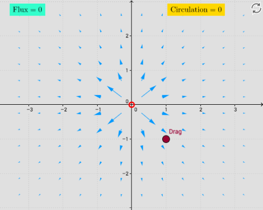
This example demonstrates the calculation and visualization of flux and circulation of a vector field within a square region, including the influence of a source. Key math concepts involve vector fields, flux, circulation, derivatives, integrals, and parametric equations. GeoGebra commands used include Sequence, Line, Circle, CurveCartesian, Derivative, Sum, Segment, Distance, and Polygon. Suitable for high school and above students learning vector calculus and field theory.
GeoGebra Commands & Parameters
Sequence(Sequence[Vector[(j, k), (j + (scale * F_1(j, k)), k + (scale * F_2(j, k)))], j, xmin, xmax, xstep], k, ymin, ymax, ystep) → vFieldLine(I, xAxis) → fLine(J, xAxis) → gLine(K, xAxis) → hSequence(Segment[Rotate[curlPt - (0.2, 0), k + curlAngle, curlPt], Rotate[curlPt + (0.2, 0), k + curlAngle, curlPt]], k, 0, 2.0944, 1.0472) → spokesCircle(divPt, 0.2) → divGlowCircleCurveCartesian((t * x(L)) + ((1 - t) * x(L)), (t * (y(L) + Length)) + ((1 - t) * y(L)), t, 0, 1) → path_{s1}CurveCartesian((t * (x(L) - Length)) + ((1 - t) * x(L)), (t * (y(L) + Length)) + ((1 - t) * (y(L) + Length)), t, 0, 1) → path_{s2}CurveCartesian((t * (x(L) - Length)) + ((1 - t) * (x(L) - Length)), (t * y(L)) + ((1 - t) * (y(L) + Length)), t, 0, 1) → path_{s3}CurveCartesian((t * x(L)) + ((1 - t) * (x(L) - Length)), (t * y(L)) + ((1 - t) * y(L)), t, 0, 1) → path_{s4}Derivative(path_{s1}) → Dpath_{s1}Derivative(path_{s2}) → Dpath_{s2}Derivative(path_{s3}) → Dpath_{s3}Derivative(path_{s4}) → Dpath_{s4}Sum(Sequence[(((F_1(x(path_{s1}(i + dS / 2)), y(path_{s1}(i + dS / 2))), F_2(x(path_{s1}(i + dS / 2)), y(path_{s1}(i + dS / 2)))) * (y(Dpath_{s1}(i + dS / 2)), (-x(Dpath_{s1}(i + dS / 2))))) * dS), i, 0, 1 - dS, dS]) → Flux_{s1}Sum(Sequence[(((F_1(x(path_{s2}(i + dS / 2)), y(path_{s2}(i + dS / 2))), F_2(x(path_{s2}(i + dS / 2)), y(path_{s2}(i + dS / 2)))) * (y(Dpath_{s2}(i + dS / 2)), (-x(Dpath_{s2}(i + dS / 2))))) * dS), i, 0, 1 - dS, dS]) → Flux_{s2}Sum(Sequence[(((F_1(x(path_{s3}(i + dS / 2)), y(path_{s3}(i + dS / 2))), F_2(x(path_{s3}(i + dS / 2)), y(path_{s3}(i + dS / 2)))) * (y(Dpath_{s3}(i + dS / 2)), (-x(Dpath_{s3}(i + dS / 2))))) * dS), i, 0, 1 - dS, dS]) → Flux_{s3}Sum(Sequence[(((F_1(x(path_{s4}(i + dS / 2)), y(path_{s4}(i + dS / 2))), F_2(x(path_{s4}(i + dS / 2)), y(path_{s4}(i + dS / 2)))) * (y(Dpath_{s4}(i + dS / 2)), (-x(Dpath_{s4}(i + dS / 2))))) * dS), i, 0, 1 - dS, dS]) → Flux_{s4}Sum(list1, (s * 4)) → TTSum(Sequence[((path_{s1}(i + dS) - path_{s1}(i)) * (F_1(x(path_{s1}(i + dS / 2)), y(path_{s1}(i + dS / 2))), F_2(x(path_{s1}(i + dS / 2)), y(path_{s1}(i + dS / 2))))), i, 0, s - dS, dS]) → Circ_1Sum(Sequence[((path_{s2}(i + dS) - path_{s2}(i)) * (F_1(x(path_{s2}(i + dS / 2)), y(path_{s2}(i + dS / 2))), F_2(x(path_{s2}(i + dS / 2)), y(path_{s2}(i + dS / 2))))), i, 0, s - dS, dS]) → Circ_2Sum(Sequence[((path_{s3}(i + dS) - path_{s3}(i)) * (F_1(x(path_{s3}(i + dS / 2)), y(path_{s3}(i + dS / 2))), F_2(x(path_{s3}(i + dS / 2)), y(path_{s3}(i + dS / 2))))), i, 0, s - dS, dS]) → Circ_3Sum(Sequence[((path_{s4}(i + dS) - path_{s4}(i)) * (F_1(x(path_{s4}(i + dS / 2)), y(path_{s4}(i + dS / 2))), F_2(x(path_{s4}(i + dS / 2)), y(path_{s4}(i + dS / 2))))), i, 0, s - dS, dS]) → Circ_4Sum(list2, (4 * s)) → TT_2Segment(path_{s1}(0.5), path_{s1}(0.5 + 0.01)) → arrw01Segment(path_{s2}(0.5), path_{s2}(0.5 + 0.01)) → arrw02Segment(path_{s3}(0.5), path_{s3}(0.5 + 0.01)) → arrw03Segment(path_{s4}(0.5), path_{s4}(0.5 + 0.01)) → arrw04Distance(L, (0, 0)) → condPolygon(L, M, 4) → poly1, i, j, k, l, N, O
AI Drawing Prompt Reference
Draw a square region with a vector field shown as arrows at grid points. Mark the four sides of the square with curved paths and direction arrows. Place a small circle at the center to indicate a source, with radial spokes around it. Display numerical labels for flux and circulation near the square, and use small arrows to show flow direction. The figure illustrates flux and circulation of a vector field.
The prompt above was compiled from the original drawing commands and is for reference only.