
Flux Across a Line Segment in a Vector Field
Loading the math board and drawing, please wait…
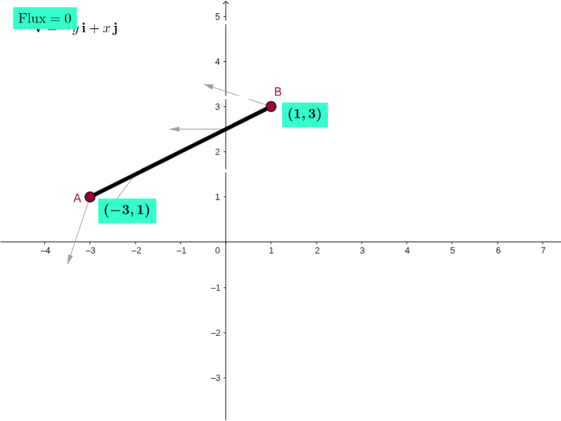
This GeoGebra example demonstrates flux across a line segment or curve in a vector field, visualizing field direction and magnitude with arrows, particles, pathlines, and a scaled grid. It covers vector fields, line integrals/curve integrals, flux, divergence, curl, parametric curves, and numerical summation. Construction uses CurveCartesian to draw field-related curves, Sequence and Point to generate sample particles or path points, Line, Ray, and Midpoint to build segments and directions, Derivative and Sum to approximate local change and flux, and Circle, Sector, Mirror, and Translate to render arrows, sectors, and symmetric helpers. Objects such as vField, particlesList, pathlinesList, curl, div, and spokes organize the animation and labels. It is suitable for advanced high-school calculus, university vector calculus, and demonstrations of flux, divergence, curl, and line-integral geometry.
GeoGebra Commands & Parameters
Circle((0, 0), 16) → kSequence(Sequence[Vector[(j, k), (j + (scale * F_1(j, k)), k + (scale * F_2(j, k)))], j, xmin, xmax, xstep], k, ymin, ymax, ystep) → vFieldSequence(((x(Element[inicialPts, i]) * cos((w * time))) - (y(Element[inicialPts, i]) * sin((w * time))), (x(Element[inicialPts, i]) * sin((w * time))) + (y(Element[inicialPts, i]) * cos((w * time)))), i, 1, 8) → particlesListSequence(CurveCartesian[(x(Element[inicialPts, i]) * cos((w * t))) - (y(Element[inicialPts, i]) * sin((w * t))), (x(Element[inicialPts, i]) * sin((w * t))) + (y(Element[inicialPts, i]) * cos((w * t))), t, 0, time], i, 1, 8) → pathlinesListCircle(divPt, 0.5) → divGlowCircleSequence(Segment[Rotate[curlPt - (0.5, 0), k + curlAngle, curlPt], Rotate[curlPt + (0.5, 0), k + curlAngle, curlPt]], k, 0, 2.0944, 1.0472) → spokesMidpoint(I, J) → MidPointLine(K, xAxis) → gLine(L, xAxis) → hLine(M, xAxis) → iCurveCartesian((t * x(J)) + ((1 - t) * x(I)), (t * y(J)) + ((1 - t) * y(I)), t, 0, 1) → pathTestCurveCartesian(x(pathTest(i)), y(pathTest(i)), i, 0, s) → partPathTestDerivative(pathTest) → DpathSum(Sequence[(((F_1(x(pathTest(i + dS / 2)), y(pathTest(i + dS / 2))), F_2(x(pathTest(i + dS / 2)), y(pathTest(i + dS / 2)))) * (y(Dpath(i + dS / 2)), (-x(Dpath(i + dS / 2))))) * dS), i, 0, s - dS, dS]) → FluxTestSequence(Vector[pathTest(i), pathTest(i) + ((scale * F_1(x(pathTest(i)), y(pathTest(i)))), (scale * F_2(x(pathTest(i)), y(pathTest(i)))))], i, 0, s, 0.25) → PathVectorsPoint(k) → PRay((0, 0), N) → dTranslate(normalvector_1, PtPath_1) → uSector(k, Q, N) → pMirror(u, PtPath_1) → u'
AI Drawing Prompt Reference
Describe a graphical representation of flux in a vector field. Include a vector field (vField) composed of curves, particles (particlesList) moving along paths, pathlines (pathlinesList) showing particle trajectories, divergence (divGlowCircle), and curl (curl) represented by spokes. A scaled grid (scaled grid) provides reference. Arrows (Vector) indicate direction; test paths (pathTest) and derivatives (Dpath) are used to calculate flux (FluxTest); path vectors (PathVectors) show particle motion directions. Construction order: first draw the grid and vector field, then add particles and pathlines, followed by divergence and curl, and finally arrows and flux calculations.
The prompt above was compiled from the original drawing commands and is for reference only.