
Finding Polynomial Roots Using Iteration
Loading the math board and drawing, please wait…
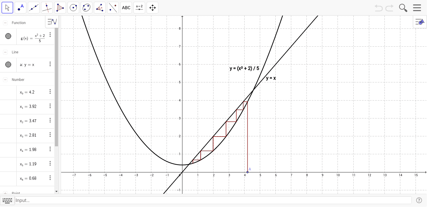
This example demonstrates visually solving polynomial equations by iterating methods, involving stochastic processes, secant lines, exponentiation, and polynomial root properties. Constructed with GeoGebra commands like Point and Segment, objects include g, a, A, x_0-x_6, c-t for visualizing the iterative process. Suitable for high school and above students learning numerical analysis and root-finding techniques.
GeoGebra Commands & Parameters
Point(xAxis) → ASegment(A, (x(A), x_1)) → bSegment((x_0, g(x_0)), (x_1, x_1)) → cSegment((x_1, g(x_1)), (x_2, x_2)) → dSegment((x_3, g(x_3)), (x_3, x_3)) → eSegment((x_4, g(x_4)), (x_4, x_4)) → fSegment((x_5, g(x_5)), (x_5, x_5)) → hSegment((x_6, g(x_6)), (x_6, x_6)) → iSegment((x_1, x_1), (x_1, g(x_1))) → jSegment((x_2, x_2), (x_2, g(x_2))) → kSegment((x_3, x_3), (x_3, g(x_3))) → lSegment((x_4, x_4), (x_4, g(x_4))) → mSegment((x_5, x_5), (x_5, g(x_5))) → nSegment((x_6, x_6), (x_6, g(x_6))) → pSegment((x_2, g(x_2)), (x_3, x_3)) → qSegment((x_3, g(x_3)), (x_4, x_4)) → rSegment((x_4, g(x_4)), (x_5, x_5)) → sSegment((x_5, g(x_5)), (x_6, x_6)) → t
AI Drawing Prompt Reference
Draw a function graph and visualize solving polynomial roots using iteration. Start from a point on the x-axis, connect it to a series of points x_1 to x_6, and draw vertical line segments from each x_i to the function value g(x_i). Then, connect each x_i to the next x_{i+1} with horizontal line segments to form a polyline. Also, draw vertical line segments from each g(x_i) down to x_i, creating segments from the function graph to the x-axis. Finally, connect adjacent g(x_i) and x_{i+1} points to form lines that connect the polyline, showing the iterative process.
The prompt above was compiled from the original drawing commands and is for reference only.