
Extended Law of Sines Demonstration
Loading the math board and drawing, please wait…
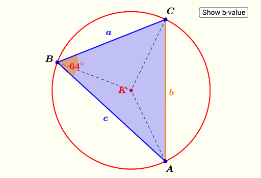
This example dynamically illustrates the extended application of the Law of Sines in arbitrary triangles, visually presenting the relationship between side lengths and sine values of angles. Core mathematical concepts include the Law of Sines, geometric properties of triangles, unit circle, vectors, and geometric constructions. Construction highlights involve GeoGebra commands such as Intersect, Point, Circle, Line, Polygon, OrthogonalLine, Angle, Segment, Ray, Vector, AngularBisector, and Midpoint. Suitable for high school and above learners to deepen understanding of the integration of trigonometric functions and geometric constructions.
GeoGebra Commands & Parameters
Intersect(xAxis, yAxis) → KPoint(xAxis) → UCircle(K, U) → circPoint(circ) → APoint(circ) → CPoint(circ) → BLine(B, C) → h_1Polygon(B, C, A) → poly1, a, b, cOrthogonalLine(A, a) → mLine(B, A) → g_1OrthogonalLine(C, c) → lLine(C, A) → f_1OrthogonalLine(B, b) → nAngle(B, A, C) → αAngle(A, B, C) → βAngle(B, C, A) → γSegment(B, K) → fSegment(A, K) → gSegment(C, K) → hRay(K, A) → iRay(K, C) → jCircle(K, 1 + e) → dRay(K, B) → kIntersect(d, k, 1) → DIntersect(d, j, 1) → EIntersect(d, i, 1) → FIntersect(n, f_1) → JIntersect(l, g_1) → HVector(K, H) → uVector(K, J) → vIntersect(m, h_1) → GVector(K, G) → wAngularBisector(A, B, C) → pCircle(B, Min[{(2 * e), (0.4 * a), (0.4 * c)}]) → qIntersect(q, p, 2) → NLine(A, (1 / 2 * (B + C))) → rIntersect(r, a) → OVector(A, G) → sMidpoint(c) → QMidpoint(b) → RVector(C, H) → tVector(B, J) → u_1Polygon({Corner[1], Corner[2], Corner[3], Corner[4]}) → poly2Circle(K, 1) → c_1