
Exponential Decay (Growth) Demo
Loading the math board and drawing, please wait…
In collections
Geom. & Alg.: Exponential Functions & Logarithms
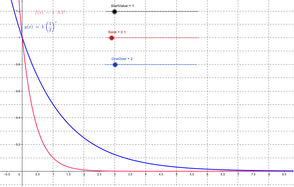
This example demonstrates the mathematical model of exponential decay (growth) and its graphical representation. Key concepts include exponential functions, decay rates, and operations with fractions and decimals. Construction highlights involve GeoGebra commands like StartValue (initial value), Base (base), f (function), OneOver (reciprocal), and g (auxiliary function). Suitable for high school mathematics education to understand exponential change patterns and the impact of parameters on function graphs.
GeoGebra Commands & Parameters
Numeric StartValue(1.0)Numeric Base(0.1)f(x) = StartValue * Base^(x)Numeric OneOver(2.0)g(x) = StartValue * (1 / OneOver)^(x)
AI Drawing Prompt Reference
Plot the graph of exponential decay (growth), with an initial value of 1.0 and a decay rate of 0.1, using the function f(x) = 1.0 * 0.1^x. Then plot an auxiliary function g(x) with an initial value of 1.0 and a decay rate of 1/2.0, using the function g(x) = 1.0 * (1/2.0)^x.
The prompt above was compiled from the original drawing commands and is for reference only.