
Exploring Polar Curve Intersections
Loading the math board and drawing, please wait…
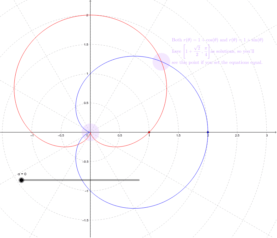
This example demonstrates how to explore the intersections of two polar curves using GeoGebra. Key mathematical concepts include polar coordinate equations, curve intersection calculations, and geometric constructions. Construction highlights involve using commands like CurveCartesian for Cartesian curves, Angle and Point for defining angles and points, and Circle and Ray for geometric shapes. Suitable for high school and above learners to understand geometric relationships and computational methods in polar coordinate systems.
GeoGebra Commands & Parameters
CurveCartesian((r_1(t) * cos(t)), (r_1(t) * sin(t)), t, 0, 6.283185307179586) → aCurveCartesian((r_2(t) * cos(t)), (r_2(t) * sin(t)), t, 0, 6.283185307179586) → bAngle((2, 0), (0, 0), D) → θPoint(a) → CCircle(C, 0.15) → dCircle(O, 0.15) → eCircle(O, 0.15) → fCircle(O, 0.15) → gRay(O, D) → c
AI Drawing Prompt Reference
Draw the intersection points of two polar curves. First, draw two curves defined by r1(t) * cos(t) and r1(t) * sin(t), and r2(t) * cos(t) and r2(t) * sin(t). Then, mark the intersection point C with a small circle. Also, draw a ray from the origin O to point C, and add some small circles as auxiliary markers. Ensure the graph is clear to show geometric relationships in polar coordinates.
The prompt above was compiled from the original drawing commands and is for reference only.