
Experimental Probability Spinner by Aedamar Frawley
Loading the math board and drawing, please wait…
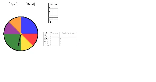
This example demonstrates the concept of experimental probability. It simulates a random spin of a spinner to illustrate basic principles of probability and statistics. Commands such as CountIf, Circle, Rotate, Vector, Line, OrthogonalLine, Intersect, CircleSector, Midpoint, IsInRegion, Sum, Element, and TableText are used to construct a dynamic model of experimental probability. Suitable for middle school and above students to learn probability and statistics.
GeoGebra Commands & Parameters
CountIf(x ≟ "orange", B2:B11) → E7CountIf(x ≟ "violet", B2:B11) → E6CountIf(x ≟ "green", B2:B11) → E5CountIf(x ≟ "yellow", B2:B11) → E4CountIf(x ≟ "red", B2:B11) → E3CountIf(x ≟ "blue", B2:B11) → E2Circle(A, B) → cRotate(S0, ((-a))°, A) → CVector(A, C) → uLine(B, A) → bOrthogonalLine(A, b) → eIntersect(c, e) → D, ECircleSector(A, E, B) → fIntersect(c, b) → F, GMidpoint(G, E) → HLine(A, H) → gIntersect(c, g) → I, JCircleSector(A, J, E) → hCircleSector(A, G, J) → kCircleSector(A, D, G) → pCircleSector(A, I, D) → qCircleSector(A, B, I) → rIsInRegion(C, f) → iIsInRegion(C, h) → jSum(Sequence[(IsInRegion[C, Element[liste2, k]] * k), k, 1, 6]) → mElement(liste1, m) → texte1TableText({{A1, B1}, {A2, B2}, {A3, B3}, {A4, B4}, {A5, B5}, {A6, B6}, {A7, B7}, {A8, B8}, {A9, B9}, {A10, B10}, {A11, B11}}, "|_") → text1TableText({{D1, E1, F1}, {D2, E2, F2}, {D3, E3, F3}, {D4, E4, F4}, {D5, E5, F5}, {D6, E6, F6}, {D7, E7, F7}}, "|_") → text2