
Electric Field Vector Field of Two Charges
Loading the math board and drawing, please wait…
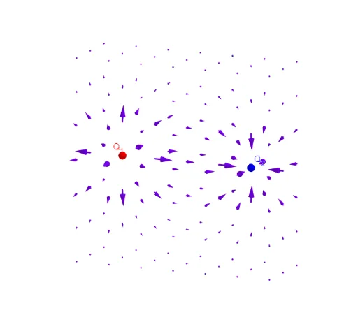
This example demonstrates the electric field vector field produced by two point charges in 3D space, using arrows to show the direction and relative magnitude of the field at sampled points. The core mathematical concepts involve Coulomb's law, vector superposition, and discrete sampling of a vector field. The construction uses GeoGebra's Sequence command to generate a grid of points, then computes the electric field vector at each point based on the charge positions Q1 and Q2, and visualizes them with Feldstärkevektoren and Richtungsvektoren objects. Sliders and parameters (t, a, g) allow interactive adjustment of charge positions and magnitudes. This is suitable for high school physics or introductory university electromagnetism courses, helping students grasp field distributions and vector field visualization.
GeoGebra Commands & Parameters
Sequence(Sequence[Sequence[(i, j, k), i, (-g), g], j, (-t), t], k, 0, (2 * g)) → PunkteSequence(Sequence[Sequence[(i, j, k) + (l * Vector[(Q_{1} * ((i, j, k) - A) / Distance[(i, j, k), A]^(3)) + (Q_{2} * ((i, j, k) - B) / Distance[(i, j, k), B]^(3))]), i, (-g), g], j, (-t), t], k, 0, (2 * g)) → FeldstärkeSequence(Sequence[Sequence[(i, j, k) + (l * UnitVector[Vector[(Q_{1} * ((i, j, k) - A) / Distance[(i, j, k), A]^(3)) + (Q_{2} * ((i, j, k) - B) / Distance[(i, j, k), B]^(3))]]), i, (-g), g], j, (-t), t], k, 0, (2 * g)) → RichtungSequence(Sequence[Sequence[Vector[Punkte(i, j, k), Feldstärke(i, j, k)], i, 1, 1 + (2 * g)], j, 1, 1 + (2 * t)], k, 1, 1 + (2 * g)) → FeldstärkevektorenSequence(Sequence[Sequence[Vector[Punkte(i, j, k), Richtung(i, j, k)], i, 1, 1 + (2 * g)], j, 1, 1 + (2 * t)], k, 1, 1 + (2 * g)) → Richtungsvektoren
AI Drawing Prompt Reference
Create a 3D vector field showing the electric field generated by two point charges. Start with a regular grid of sample points in a horizontal plane. At each grid point, compute the net electric field vector from both charges using Coulomb's law, and draw arrows to represent both the direction and relative magnitude. Additionally, draw a second set of arrows showing only the direction of the field, ignoring magnitude. The positions and charges of the two points can be adjusted interactively, as can the grid density and extent. The result is a spatial distribution of arrows illustrating how the field emanates from positive charges and terminates at negative ones.
The prompt above was compiled from the original drawing commands and is for reference only.