
Dynamic Visualization of Volume of Revolution
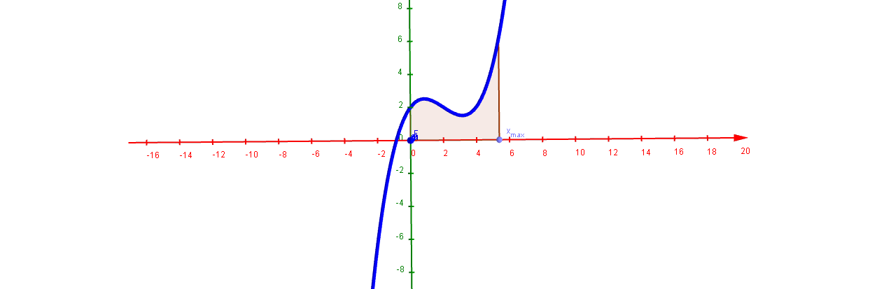
Loading the math board and drawing, please wait…
This GeoGebra example dynamically demonstrates how a plane region rotated around an axis generates a solid of revolution and how its volume is computed. The core mathematical concept is the application of definite integrals in solid geometry, specifically the disk or shell method for volume calculation. Construction highlights include: using CurveCartesian to define the parametric surface of the solid, Sequence and Append to generate layered meshes (Mesh_1, Mesh_2) for a 3D effect, Intersect, Point, Line, Circle, and Angle to construct the rotation axis and cross-sections, Polygon and Rotate to create the original plane region, and a slider (n_points) to control discretization precision, allowing users to observe how volume changes with parameters. Suitable for high school to early college calculus or solid geometry instruction, this example helps students grasp the geometric meaning behind integration for volume.
GeoGebra Commands & Parameters
Intersect(yAxis, zAxis) → APoint(xAxis) → BLine(A, B) → aCircle(a, C) → cPoint(c) → DPoint(a) → EAngle(C, A, D) → αCurveCartesian(t, (f(t) * cos(α)), (f(t) * sin(α)), t, 0, x(E)) → bSequence(Circle[((q * x(E) / Mesh_2), 0, 0), f((q * x(E) / Mesh_2)), x + 0z = 0], q, 0, Mesh_2) → list2Sequence(CurveCartesian[t, (f(t) * cos(((2 * π) * q / Mesh_1))), (f(t) * sin(((2 * π) * q / Mesh_1))), t, 0, x(E)], q, 1, Mesh_1) → list1Append((x(E), 0), Append[(0, 0), Sequence[((x(E) * q / n_{points}), f((x(E) * q / n_{points}))), q, 0, n_{points}]]) → liste1Polygon(liste1) → poly1Rotate(poly1, α, a) → poly1'