
Dynamic Quadrilateral Loci - Race Track Model
Loading the math board and drawing, please wait…
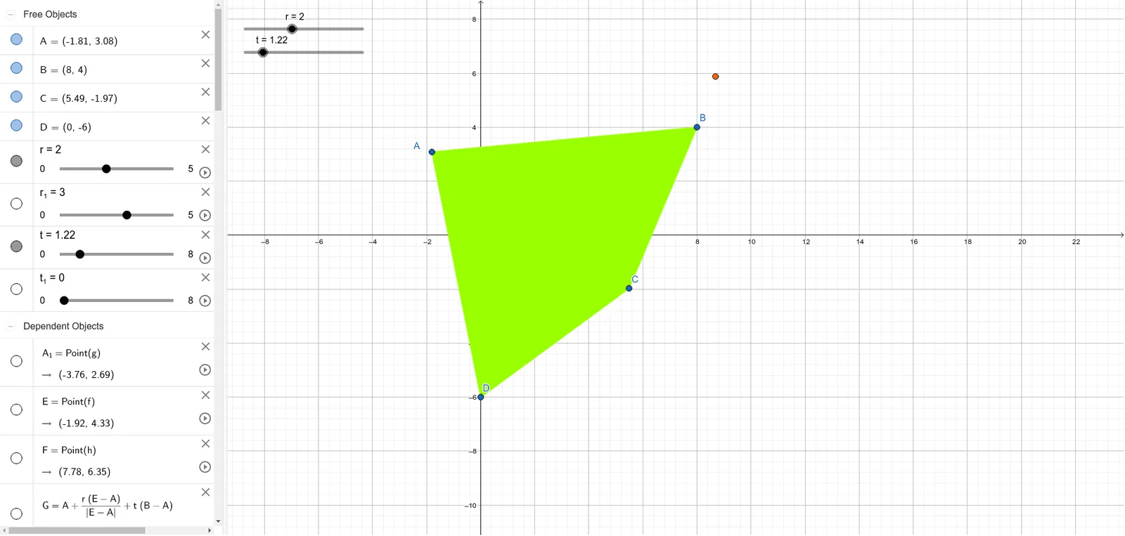
① This example uses a dynamic quadrilateral to simulate a race track, demonstrating how loci are formed by moving vertices and tracking related points such as intersections and perpendicular feet. ② Core math concepts include quadrilateral properties, perpendicular lines, angles, loci, and parametric changes in dynamic geometry. ③ Construction highlights: using GeoGebra commands like Polygon to build quadrilateral ABCD, OrthogonalLine for perpendiculars, Point and Angle for dynamic elements, and numerous auxiliary objects (r, t, f, g, h, etc.) to create complex relationships that generate the final locus curves. ④ Suitable for middle/high school geometry classes, dynamic demonstrations of locus concepts, and as material for math experiments or inquiry-based learning, helping students intuitively grasp geometric transformations and locus generation.
GeoGebra Commands & Parameters
Polygon(A, B, C, D) → q1, a_1, c_1, d_1, b_1OrthogonalLine(A, a_1) → fOrthogonalLine(A, b_1) → gOrthogonalLine(B, a_1) → hOrthogonalLine(B, c_1) → iOrthogonalLine(C, c_1) → jOrthogonalLine(C, d_1) → kOrthogonalLine(D, d_1) → lOrthogonalLine(D, b_1) → mPoint(f) → EPoint(h) → FPoint(i) → HPoint(k) → JPoint(m) → LOrthogonalLine(B, yAxis) → nAngle(H, B, F) → αPoint(n) → OAngle(H, B, O) → βOrthogonalLine(C, yAxis) → pOrthogonalLine(D, yAxis) → qOrthogonalLine(A, yAxis) → sPoint(p) → PAngle(J, C, P) → γPoint(j) → QAngle(J, C, Q) → δPoint(l) → SPoint(q) → TPoint(q) → VAngle(L, D, V) → εAngle(L, D, S) → ζPoint(s) → ZPoint(g) → A_1Angle(Z, A, A_1) → ηAngle(E, A, A_1) → θ