
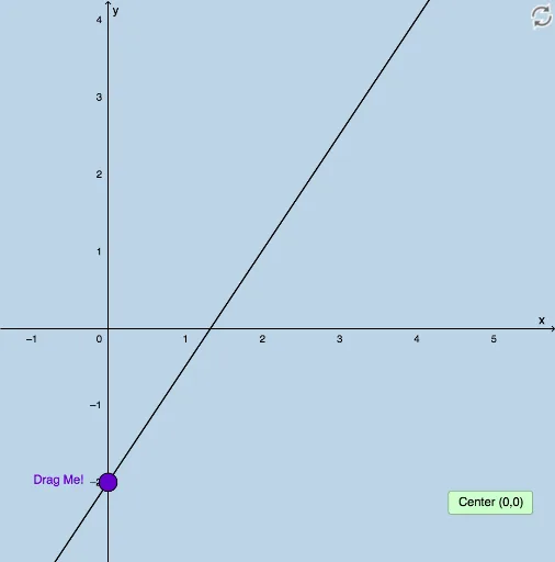
Dynamic Illustration of Line Equation
Loading the math board and drawing, please wait…
This example dynamically illustrates the equation of a non-vertical line. Key mathematical concepts include linear equations and geometric transformations. Using GeoGebra commands such as Vector, Translate, and Dilate, the dynamic changes in the line's position and scaling can be observed. Suitable for students at the junior high school level and above to learn about linear equations and geometric transformations.
GeoGebra Commands & Parameters
Vector((0, 0), (1, 0)) → uTranslate(A, u) → A'Dilate(A, If[0 < o ≤ 1, 1 - o, 0], A') → A'_1Dilate(A'_1, If[1 < o ≤ 2, 2 - o, 0], B) → HDilate((0, 0), If[-1 < o ≤ 0, (-o), 0], A) → D_1Translate(G, u) → G'Translate(B, u) → B'Translate(C, u) → C'Translate(D, u) → D'Polygon(A, A', B) → poly1, b, a_1, a'Polygon(B, B', C) → poly2, c, b_1, b'Polygon(C, C', D) → poly3, d, c_1, c'Polygon(D, D', E) → poly4, e, d_1, d'Dilate(B, If[0 < o ≤ 1, 1 - o, 0], B') → B'_1Dilate(C, If[0 < o ≤ 1, 1 - o, 0], C') → C'_1Dilate(D, If[0 < o ≤ 1, 1 - o, 0], D') → D'_1Segment(A, A'_1) → pSegment(B, B'_1) → qSegment(C, C'_1) → rSegment(D, D'_1) → sDilate(A'_1, If[2 < o ≤ 3, 3 - o, 0], B'_1) → IVector(A'_1, I) → vTranslate(A'_1, v) → JTranslate(H, v) → H'Dilate(B'_1, If[3 < o ≤ 4, 4 - o, 0], C'_1) → KVector(B'_1, K) → wTranslate(J, w) → J'Translate(H', w) → H''Dilate(C'_1, If[4 < o ≤ 5, 5 - o, 0], D'_1) → MVector(C'_1, M) → u_1Translate(J', u_1) → J''Translate(H'', u_1) → H'''Translate(L, u) → L'Translate(F, u) → F'Line(A, B) → f_1IntegralBetween(f, g, 0, 1) → e_1Translate(O, u) → O'IntegralBetween(f, g_1, 1, 2) → h_1IntegralBetween(f, h, 2, 3) → i_1Dilate(O, If[0 < p_1 ≤ 1, 1 - p_1, 0], O') → O'_1Dilate(L, If[0 < p_1 ≤ 1, 1 - p_1, 0], L') → L'_1Dilate(G, If[0 < p_1 ≤ 1, 1 - p_1, 0], G') → G'_1Segment(G, G'_1) → k_1Segment(O, O'_1) → l_1Segment(L, L'_1) → m_1Dilate(G'_1, If[1 < p_1 ≤ 2, 2 - p_1, 0], O) → PSegment(G'_1, P) → q_1Midpoint(O'_1, L) → QMidpoint(L'_1, F) → RDilate(G'_1, If[2 < p_1 ≤ 3, 3 - p_1, 0], O'_1) → SVector(G'_1, S) → v_1Translate(G'_1, v_1) → TTranslate(P, v_1) → P'Segment(T, P') → j_1Dilate(G'_1, If[3 < p_1 ≤ 4, 4 - p_1, 0], Q) → UVector(G'_1, U) → w_1Translate(G'_1, w_1) → VTranslate(P, w_1) → P'_1Segment(V, P'_1) → n_1Segment(O'_1, L) → r_1Dilate(O'_1, If[4 < p_1 ≤ 5, 5 - p_1, 0], L'_1) → WVector(O'_1, W) → s_1Translate(O'_1, s_1) → ZTranslate(L, s_1) → L'_2Segment(Z, L'_2) → t_1Dilate(O'_1, If[5 < p_1 ≤ 6, 6 - p_1, 0], R) → A_1Vector(O'_1, A_1) → u_2Translate(O'_1, u_2) → B_1Translate(L, u_2) → L'_3Segment(B_1, L'_3) → f_2Segment(C_1, A) → g_2Slope(f_1) → a_2Textfield(m) → InputBox1Distance(C_1, A) → distanceC1ADistance(A'_1, H) → c_2Vector(E_1, D_1) → v_2Vector(A'_1, H) → tDistance(E_1, D_1) → distanceE1D1Vector(J, H') → w_2Vector(J', H'') → c_2Vector(J'', H''') → d_2Distance(J, C) → distanceJCDistance(J', D) → distanceJ'DDistance(J'', E) → distanceJ''E
AI Drawing Prompt Reference
Draw a non-vertical line and dynamically show its position and scaling changes. First, create a horizontal vector, then use translation and dilation operations to dynamically change the line's position and shape. Finally, draw several polygons and segments to demonstrate the line's changes at different scaling ratios.
The prompt above was compiled from the original drawing commands and is for reference only.