
Dynamic Demonstration of Polynomial Functions and Line Intersections
Loading the math board and drawing, please wait…
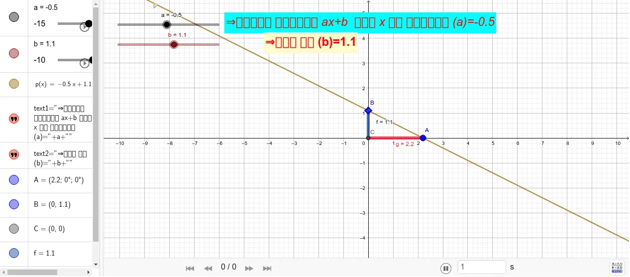
This example provides a visual exploration of the intersection points between polynomial functions and linear equations. It focuses on core mathematical concepts such as the properties of polynomial graphs, linear functions, and the algebraic determination of roots. The construction utilizes the 'Intersect' command to identify meeting points between function f and line g, and the 'Segment' command to create connecting lines, with points (A, B, C, p) and text labels (text1, text2) used for precise coordinate tracking. This tool is ideal for high school students studying function analysis, equation solving, or introductory calculus limits.
GeoGebra Commands & Parameters
Intersect(p, xAxis, 1) → AIntersect(p, yAxis, 1) → BIntersect(xAxis, yAxis) → CSegment(C, B) → fSegment(C, A) → g
AI Drawing Prompt Reference
Draw a graph with coordinate axes. Mark three intersection points A, B, and C. A is where a line meets the x-axis, B is where another line meets the y-axis, and C is where the axes intersect. Draw a line segment f from C to B and a line segment g from C to A. The graph should clearly show these points and their connections to help understand the intersection of functions and lines.
The prompt above was compiled from the original drawing commands and is for reference only.