
Dynamic Demonstration of Exponential Growth & Decay
Loading the math board and drawing, please wait…
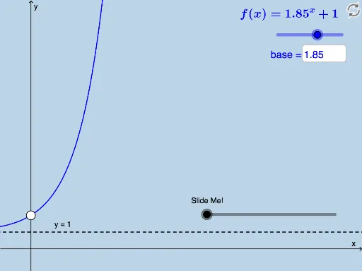
This GeoGebra example dynamically illustrates exponential growth and decay. It involves the core mathematical concept of exponential functions. Using commands like Vector, Translate, Polygon, Dilate, Segment, Line, IntegralBetween, Circle, Intersect, Rotate, Midpoint, Distance, Textfield, users can intuitively understand the properties of exponential functions. Suitable for high school mathematics education and learning.
GeoGebra Commands & Parameters
Vector((0, 0), (1, 0)) → uTranslate(G, u) → G'Translate(B, u) → B'Translate(C, u) → C'Translate(D, u) → D'Translate(A, u) → A'Polygon(A, A', B) → poly1, b, a_1, a'Polygon(B, B', C) → poly2, c, b_1, b'Polygon(C, C', D) → poly3, d, c_1, c'Polygon(D, D', E) → poly4, e, d_1, d'Dilate(A, If[0 < o ≤ 1, 1 - o, 0], A') → A'_1Dilate(B, If[0 < o ≤ 1, 1 - o, 0], B') → B'_1Dilate(C, If[0 < o ≤ 1, 1 - o, 0], C') → C'_1Dilate(D, If[0 < o ≤ 1, 1 - o, 0], D') → D'_1Segment(A, A'_1) → pSegment(B, B'_1) → qSegment(C, C'_1) → rSegment(D, D'_1) → sDilate(A'_1, If[1 < o ≤ 2, 2 - o, 0], B) → HSegment(A'_1, H) → tDilate(A'_1, If[2 < o ≤ 3, 3 - o, 0], B'_1) → IVector(A'_1, I) → vTranslate(A'_1, v) → JTranslate(H, v) → H'Segment(J, H') → t'Dilate(B'_1, If[3 < o ≤ 4, 4 - o, 0], C'_1) → KVector(B'_1, K) → wTranslate(J, w) → J'Translate(H', w) → H''Segment(J', H'') → t''Dilate(C'_1, If[4 < o ≤ 5, 5 - o, 0], D'_1) → MVector(C'_1, M) → u_1Translate(J', u_1) → J''Translate(H'', u_1) → H'''Segment(J'', H''') → t'''Translate(L, u) → L'Translate(F, u) → F'Line(A, B) → f_1IntegralBetween(f, g, 0, 1) → e_1Translate(O, u) → O'IntegralBetween(f, g_1, 1, 2) → h_1IntegralBetween(f, h, 2, 3) → i_1Dilate(O, If[0 < p_1 ≤ 1, 1 - p_1, 0], O') → O'_1Dilate(L, If[0 < p_1 ≤ 1, 1 - p_1, 0], L') → L'_1Dilate(G, If[0 < p_1 ≤ 1, 1 - p_1, 0], G') → G'_1Segment(O, O'_1) → l_1Segment(L, L'_1) → m_1Dilate(G'_1, If[1 < p_1 ≤ 2, 2 - p_1, 0], O) → PSegment(G'_1, P) → q_1Dilate(G'_1, If[2 < p_1 ≤ 3, 3 - p_1, 0], O'_1) → SVector(G'_1, S) → v_1Translate(G'_1, v_1) → TTranslate(P, v_1) → P'Segment(O'_1, L) → r_1Dilate(O'_1, If[4 < p_1 ≤ 5, 5 - p_1, 0], L'_1) → WVector(O'_1, W) → s_1Translate(O'_1, s_1) → ZTranslate(L, s_1) → L'_2Translate(G, u) → G'_2Translate(C_1, u) → F_1Translate(D_1, u) → G_1Dilate(G, If[0 < a_2 ≤ 1, 1 - a_2, 0], G'_2) → G'_3Dilate(C_1, If[0 < a_2 ≤ 1, 1 - a_2, 0], F_1) → H_1Dilate(D_1, If[0 < a_2 ≤ 1, 1 - a_2, 0], G_1) → I_1Segment(G, G'_3) → g_2Segment(C_1, H_1) → h_2Segment(D_1, I_1) → i_2Dilate(G'_2, If[1 < a_2 ≤ 2, 2 - a_2, 0], C_1) → J_1Segment(G'_2, J_1) → j_2IntegralBetween(f, g, 0, 1) → b_2IntegralBetween(f, g_1, 1, 2) → c_2IntegralBetween(f, h, 2, 3) → d_2Segment(D_1, F_1) → k_2Circle(F_1, e_2) → p_2Intersect(p_2, k_2) → K_1,Circle(K_1, e_2) → q_2Intersect(q_2, k_2) → L_1, M_1Dilate(G'_2, If[2 < a_2 ≤ 3, 3 - a_2, 0], M_1) → N_1Vector(G'_2, N_1) → v_2Translate(G'_2, v_2) → O_1Translate(J_1, v_2) → P_1Segment(O_1, P_1) → l_2Rotate(O_1, If[3 < a_2 ≤ 4, ((a_2 - 3) * π), π], K_1) → R_1Rotate(P_1, If[3 < a_2 ≤ 4, ((a_2 - 3) * π), π], K_1) → S_1Segment(R_1, S_1) → m_2Rotate(R_1, If[4 < a_2 ≤ 5, ((a_2 - 4) * π), π], L_1) → T_1Rotate(S_1, If[4 < a_2 ≤ 5, ((a_2 - 4) * π), π], L_1) → U_1Segment(T_1, U_1) → n_2Segment(M_1, D_1) → r_2Dilate(M_1, If[5 < a_2 ≤ 6, 6 - a_2, 0], G_1) → Q_1Vector(M_1, Q_1) → w_2Translate(M_1, w_2) → V_1Translate(D_1, w_2) → W_1Segment(V_1, W_1) → s_2Midpoint(W_1, E_1) → Z_1Rotate(V_1, If[6 < a_2 ≤ 7, ((a_2 - 6) * π), π], W_1) → A_2Rotate(W_1, If[6 < a_2 ≤ 7, ((a_2 - 6) * π), π], W_1) → B_2Segment(A_2, B_2) → t_2Rotate(A_2, If[7 < a_2 ≤ 8, ((a_2 - 7) * π), π], Z_1) → C_2Rotate(B_2, If[7 < a_2 ≤ 8, ((a_2 - 7) * π), π], Z_1) → D_2Segment(C_2, D_2) → f_3Translate(F, u) → F'_1Intersect(f, n, (4, 12.713506250000002)) → E_2Dilate(F, If[0 < p_1 ≤ 1, 1 - p_1, 0], F'_1) → F'_2Segment(F, F'_2) → g_3Dilate(O'_1, If[2 < p_1 ≤ 3, 3 - p_1, 0], L) → QSegment(O'_1, Q) → j_1Distance(O'_1, L) → distanceO'1LDilate(L'_1, If[3 < p_1 ≤ 4, 4 - p_1, 0], F) → RSegment(L'_1, R) → t_1Distance(L'_1, F) → distanceL'1FDilate(F'_1, If[4 < p_1 ≤ 5, 5 - p_1, 0], N) → USegment(F'_1, U) → f_2IntegralBetween(f, k_1, x(F), x(F'_1)) → w_1Distance(F'_1, N) → distanceF'1NTextfield(base) → InputBox1Segment(G, G'_1) → i_3
AI Drawing Prompt Reference
Create a dynamic demonstration of exponential growth and decay. Start by drawing the x-axis and y-axis. Then, use translation and scaling to create a series of parallel line segments to illustrate the properties of exponential functions. Next, draw the graph of the exponential function and shade the areas to represent integrals. Finally, use translation and scaling to dynamically show the process of exponential growth and decay.
The prompt above was compiled from the original drawing commands and is for reference only.