
Dynamic Construction and Area Exploration of Quadrilaterals
Loading the math board and drawing, please wait…
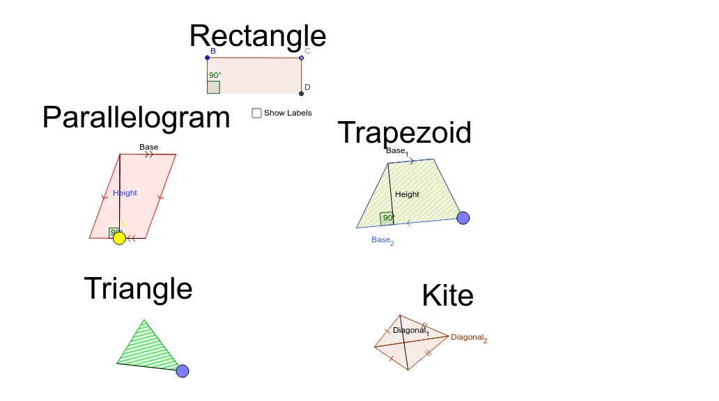
This GeoGebra example demonstrates the dynamic construction of quadrilaterals and the exploration of their area properties using fundamental geometric objects such as points, segments, lines, and polygons. Core mathematical concepts include quadrilateral area, polygon decomposition, perpendicularity, angle measurement, distance computation, and geometric transformations. The construction employs GeoGebra commands including Segment, Line, Point, Semicircle, Intersect, Polygon, OrthogonalLine, Angle, Distance, Circle, Midpoint, Ray, and Rotate, together with objects such as H_1, G_1, F_1, poly2, poly4, A, B, and C. By leveraging orthogonal lines, midpoints, rotations, and circle/semicircle intersections, the example visualizes how quadrilateral areas change under geometric constraints. It is suitable for middle school and high school plane geometry instruction, inquiry-based learning, and teacher lesson preparation.
GeoGebra Commands & Parameters
Segment(F_1, G_1) → i_2Line(H_1, i_2) → j_2Point(j_2) → I_1Semicircle(G_1, I_1) → t_2Semicircle(T, U) → c_2Segment(E, F) → eLine(G, e) → gSegment(F, G) → fLine(E, f) → hIntersect(g, h) → HPolygon(E, F, G, H) → poly2, e_1, f_1, g_1, h_1OrthogonalLine(F, h_1) → iIntersect(i, h) → JPolygon(J, F, G, H) → poly4, j_1, f_2, g_2, h_2Intersect(j_1, h_2) → QOrthogonalLine(G, f) → jIntersect(h, j) → KSegment(J, K) → mSegment(A, B) → aOrthogonalLine(B, a) → bOrthogonalLine(A, a) → cPoint(b) → COrthogonalLine(C, b) → dIntersect(c, d) → DPolygon(A, B, C, D) → poly1, a_1, b_1, c_1, d_1Angle(D, A, B) → αIntersect(h, h_1) → ISegment(E, K) → kDistance(E, J) → distanceEJDistance(F, J) → distanceFJPoint(m) → LCircle(L, distanceEJ) → pCircle(L, distanceFJ) → qLine(F, G) → lIntersect(q, l) → M, N_1Intersect(p, h) → N, OPolygon(L, M, O) → poly3, o, l_1, m_1Angle(M, L, O) → βSegment(P, H) → nSegment(F, P) → rPolygon(R, T, U) → poly5, u, r_1, tMidpoint(r_1) → VCircle(V, T) → sPoint(c_2) → WRay(W, V) → i_1Intersect(s, i_1) → Z, A_1Segment(A_1, W) → k_1Ray(R, V) → n_1Circle(V, R) → p_1Intersect(p_1, n_1) → B_1, C_1Circle(A_1, u) → s_1Circle(W, t) → t_1Intersect(s_1, t_1, 2) → D_1Polygon(W, D_1, A_1) → poly6, a_2, w, d_2Ray(R, V) → q_1OrthogonalLine(W, t) → b_2Intersect(t, b_2) → E_1Segment(W, E_1) → e_2Segment(G_1, I_1) → k_2Point(j_2) → J_1Segment(F_1, J_1) → l_2Midpoint(k_2) → K_1Circle(K_1, I_1) → p_2Point(t_2) → L_1Ray(L_1, K_1) → m_2Intersect(p_2, m_2) → M_1, O_1Angle(G_1, I_1, H_1) → γRotate(K_1, γ, L_1) → P_1Angle(K_1, L_1, P_1) → δRay(L_1, P_1) → n_2Angle(F_1, G_1, I_1) → εRotate(K_1, -ε, O_1) → Q_1Angle(Q_1, O_1, K_1) → ζRay(O_1, Q_1) → q_2Distance(I_1, J_1) → distanceI1J1Distance(G_1, F_1) → distanceG1F1Circle(L_1, distanceI1J1) → r_2Circle(O_1, distanceG1F1) → s_2Intersect(s_2, q_2, 1) → R_1Intersect(r_2, n_2, 1) → S_1Polygon(L_1, O_1, R_1, S_1) → poly7, l_3, o_1, r_3, s_3Polygon(J_1, F_1, G_1, I_1) → poly8, j_3, f_3, g_3, i_3OrthogonalLine(F_1, i_3) → a_3Intersect(j_2, a_3) → T_1Segment(F_1, T_1) → b_3Angle(F_1, T_1, J_1) → ηPoint(u) → Z_1Point(r_1) → A_2Segment(Z_1, A_2) → d_3Polygon(U_1, V_1, W_1) → poly9, w_1, u_1, v_1Circle(U_1, V_1) → c_3Circle(W_1, V_1) → e_3Intersect(c_3, e_3, 2) → B_2Polygon(U_1, B_2, W_1) → poly10, w_2, u_2, b_4Segment(V_1, B_2) → h_3
AI Drawing Prompt Reference
Create a dynamic construction of quadrilaterals and their area exploration. Start with points and segments to form quadrilateral sides, then add perpendicular lines, intersections, and circles or semicircles to build multiple polygons. Visualize how areas change under orthogonal constraints, midpoints, and rotations, including angle and distance measurements to illustrate geometric relationships for educational purposes.
The prompt above was compiled from the original drawing commands and is for reference only.