
Double Slit Experiment and Hyperbola
Loading the math board and drawing, please wait…
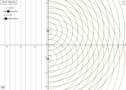
This example demonstrates the geometric relationship between wavefront propagation and hyperbolas in the double-slit experiment. Core math concepts include 3D vectors, rotation, solid geometry, differential and integral calculus. Construction highlights: Point and Sequence commands are used to create points and sequences, involving parameters like r, λ, WaveletsA, WaveletsB for wave sources, and TraceMax, showTraceBtn, showTrace for trace display. Suitable for high school students and math enthusiasts studying spatial geometry and wave theory.
GeoGebra Commands & Parameters
Point(yAxis) → ASequence(CircleArc[A, A - (0, Mod[r + (n * λ), (num * λ)]), A + (0, Mod[r + (n * λ), (num * λ)])], n, 0, num - 1) → WaveletsASequence(CircleArc[B, B - (0, Mod[r + (n * λ), (num * λ)]), B + (0, Mod[r + (n * λ), (num * λ)])], n, 0, num - 1) → WaveletsBSequence(Line[((-Mod[(n * λ) - r, (num * λ)]), 0), yAxis], n, 0, num - 1) → WavesIncomingSequence(Sequence[Intersect[Element[WaveletsA, j], Element[WaveletsB, k]], j, 1, num / 2], k, 1, num / 2) → TraceMax
AI Drawing Prompt Reference
Draw a geometric diagram of the double-slit experiment showing wavefront propagation and hyperbolas. Place two points on the vertical axis as wave sources. From each source, emit multiple circular arcs representing wavefronts of different wavelengths, with radii varying by a parameter and taken modulo. From the left, draw a series of parallel lines representing incoming waves. At the intersections of the two sets of arcs, mark all possible interference maxima points, which form hyperbolic trajectories. The overall figure includes wave sources, circular wavefronts, incoming wave lines, and intersection trajectories, illustrating wave geometry and calculus concepts in 3D space.
The prompt above was compiled from the original drawing commands and is for reference only.