
Differential Equations and Slope Fields Link Demo
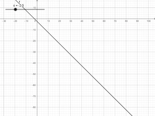
Loading the math board and drawing, please wait…
This GeoGebra example illustrates the dynamic relationship between a first‑order differential equation and its slope field. It visualizes how solution curves follow the direction field, highlighting concepts such as existence and uniqueness of solutions, initial value problems, and qualitative analysis. Construction uses the `SlopeField` command to create the direction field object `o` and `SolveODE` (or `Integral`) to plot solution curves as object `f`, with a slider controlling the initial condition for interactive exploration. Suitable for high‑school calculus electives, introductory university calculus courses, and teachers seeking an interactive classroom demonstration.
GeoGebra Commands & Parameters
Numeric o(-2.5)y = (-x) + o
AI Drawing Prompt Reference
Draw a slope field graph with a direction field and a solution curve. The direction field consists of a series of slope lines, and the solution curve follows it from an initial condition. The construction order is to first draw the direction field, then the solution curve, and set a slider to control the initial condition for interactive exploration.
The prompt above was compiled from the original drawing commands and is for reference only.