
Differential Equation Visualization
Loading the math board and drawing, please wait…
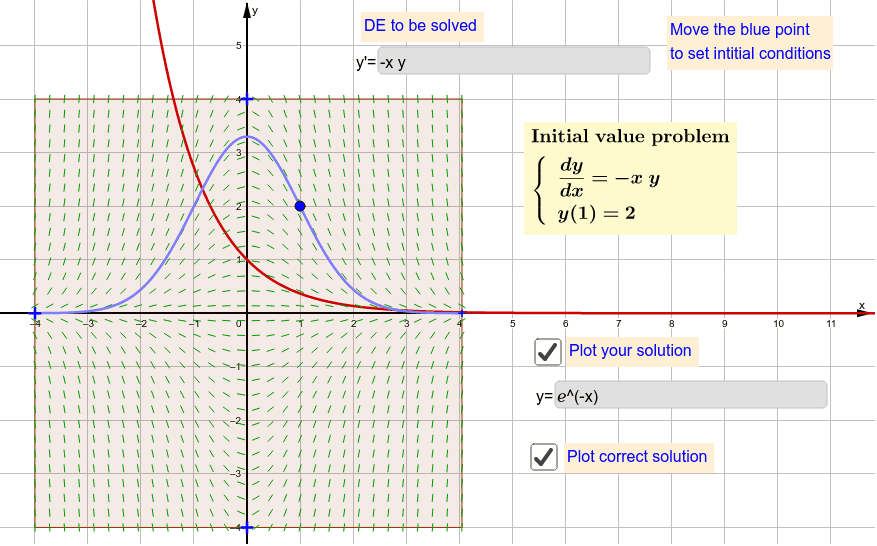
This example demonstrates the solution and direction field of differential equations through dynamic graphics. Core math concepts include differential equations, direction fields, slope fields, and solution curves. Construction highlights involve commands like Textfield, Point, OrthogonalLine, Intersect, Polygon, SlopeField, SolveODE to create an interactive interface for equation solving and visualization. Suitable for high school students and beginners in calculus learning differential equation theory.
GeoGebra Commands & Parameters
Textfield(f) → InputBox1Point(xAxis) → APoint(xAxis) → BPoint(yAxis) → CPoint(yAxis) → DOrthogonalLine(A, xAxis) → aOrthogonalLine(B, xAxis) → bOrthogonalLine(C, yAxis) → cOrthogonalLine(D, yAxis) → dIntersect(a, d) → EIntersect(a, c) → FIntersect(b, c) → GIntersect(b, d) → HPolygon(E, F, G, H) → poly1, e, f_1, g, hSlopeField(f, 30, 0.5, xmin, ymin, xmax, ymax) → slopefield1SolveODE(f, x0, y0, xmin, step) → yLeftSolveODE(f, x0, y0, xmax, step) → yRightTextfield(guess) → InputBox2