
Demonstrating Linear Equations
Loading the math board and drawing, please wait…
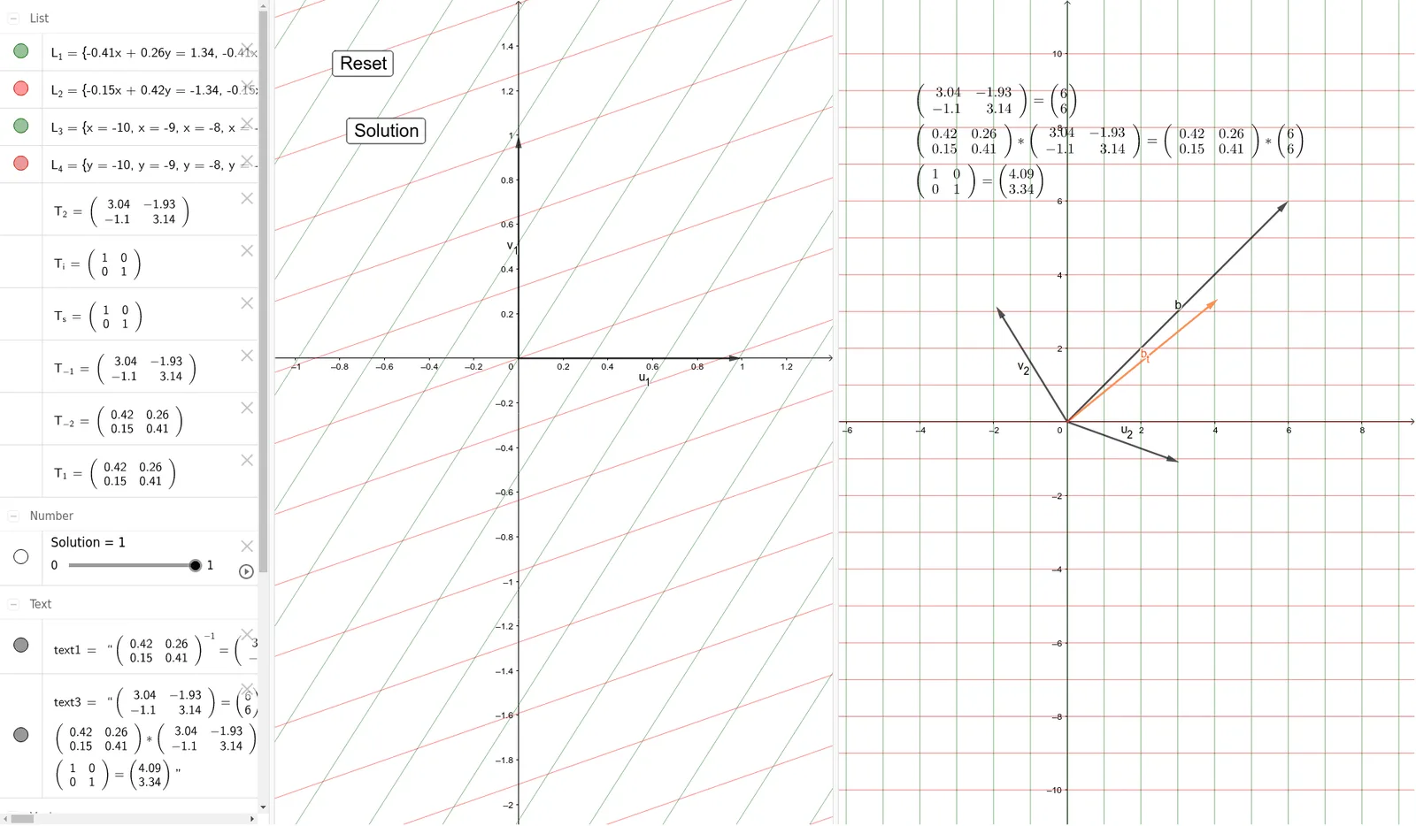
This example visually demonstrates solving systems of linear equations using vectors and geometric constructs. It involves core math concepts like linear equations, vector operations, and coordinate geometry. GeoGebra commands used include Vector, Invert, Sequence, with objects like Solution, u_i, v_i, T_i. Ideal for high school mathematics education to understand the geometric representation and solution methods of linear equations.
GeoGebra Commands & Parameters
Vector((3.0406485038772604, -1.0975096046860273)) → u_2Vector((-1.9308039341698673, 3.142269763570411)) → v_{2}Invert(T_2) → T_{-2}Vector((0, 1)) → v_{1}Vector((1, 0)) → u_{1}Sequence(Line[(T_{1} * (i, 0)), (T_{1} * (i, 1))], i, -10, 10, 1) → L_1Sequence(Line[(T_{1} * (0, i)), (T_{1} * (1, i))], i, -10, 10, 1) → L_2Invert(T_{1}) → T_{-1}Vector((6, 6)) → bSequence(Line[(T_s * (i, 0)), (T_s * (i, 1))], i, -10, 10, 1) → L_3Sequence(Line[(T_s * (0, i)), (T_s * (1, i))], i, -10, 10, 1) → L_4