
Damped Oscillation System Demo
Loading the math board and drawing, please wait…
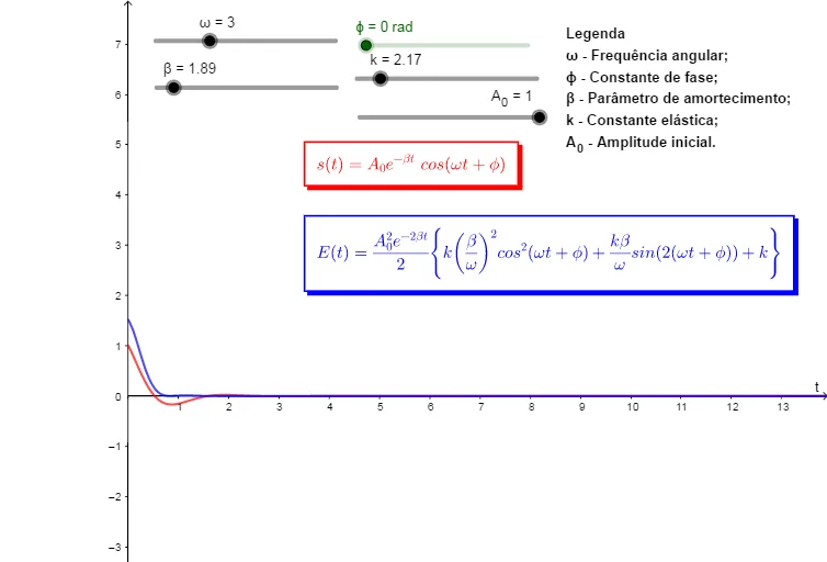
This example demonstrates the motion trajectory and energy variation of a damped oscillation system. Core mathematical concepts include calculus, differential equations, exponential functions, function graphs, and integral calculations. Key GeoGebra commands/objects used are: ϕ (phase), ω (angular frequency), β (damping coefficient), A_0 (initial amplitude), s (time), k (spring constant), E (energy), and text elements text1, text2, text3. Suitable for high school students and math enthusiasts studying vibration and wave theories.
GeoGebra Commands & Parameters
Angle ϕ(0)Numeric ω(3)Numeric β(1.889)Numeric A_0(1)s(t) = If[0 ≤ t ≤ Infinity, ((A_0 * ℯ^(((-β) * t))) * cos((ω * t) + ϕ))]Numeric k(2.17)E(t) = If[0 ≤ t ≤ Infinity, (((A_0^(2) * ℯ^(((-2 * β) * t)))) / 2 * ((((k * β)) / ω * sin((2 * ((ω * t) + ϕ)))) + ((k * (β / ω)^(2)) * cos((ω * t) + ϕ)) + k))]
AI Drawing Prompt Reference
Draw a graph of a damped oscillation system. The graph should show a displacement curve that changes over time, influenced by initial amplitude, damping coefficient, and angular frequency. The curve should indicate a gradual decay of oscillation. Also, include a graph of energy variation to show how energy decreases over time. Ensure the graph is clear and labels key parameters like initial amplitude, damping coefficient, and angular frequency.
The prompt above was compiled from the original drawing commands and is for reference only.