
Cube Nets (11 Patterns)
Loading the math board and drawing, please wait…
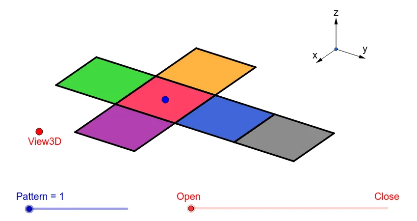
① This example demonstrates all 11 distinct nets of a cube, showing the correspondence between the 3D solid and its 2D unfolded patterns through an interactive 3D view. ② Core mathematical concepts include solid geometry, surface nets of a cube, spatial visualization, transformations between plane and solid, and symmetry. ③ Construction highlights: The GeoGebra commands used include Vector, Translate, OrthogonalLine, Polygon, Midpoint, Segment, and Mirror, along with 3D view objects (View3D), rotation parameters (sinphi, cosphi, sintheta, costheta), and multiple auxiliary points (A, P, O, etc.) and faces (poly1). The different net layouts are generated via translations and reflections. ④ Suitable for middle school to high school students learning solid geometry and developing spatial reasoning, as well as for teachers creating interactive lessons or students exploring all possible cube net configurations.
GeoGebra Commands & Parameters
Vector(B_1, Z) → wVector(B_1, Y) → vVector(B_1, X) → uTranslate(A, Vector[(2 * v)]) → A'Translate(P, Vector[(2 * v)]) → P'OrthogonalLine(View3D, yAxis) → a_1OrthogonalLine(View3D, xAxis) → b_1Polygon(L, K, N, M) → poly1, l, k_1, n, mPolygon(K, P, Q, N) → poly2, k_2, p, q, n_1Polygon(L, M, S, R) → poly3, l_1, m_1, s, rPolygon(N, V, W, M) → poly4, n_2, v_1, w_1, m_2Polygon(K, T, U, L) → poly5, k_3, t, u_1, l_2Polygon(B, Q, P, A) → poly6, b_2, q_1, p_1, a_2Midpoint(R, M) → DTranslate(S, Vector[(-((2 * v)))]) → S'Segment(S, C) → eTranslate(M, Vector[((-2) * v)]) → M'Segment(M, E) → fSegment(E, C) → hTranslate(N, Vector[((-2) * v)]) → N'Translate(Q, Vector[((-2) * v)]) → Q'_1Segment(Q, F) → iSegment(N, G) → jSegment(G, F) → d_1Translate(Q, Vector[((-2) * v)]) → Q'_2Translate(B, Vector[((-2) * v)]) → B'_1Segment(B, I) → e_1Segment(I, H) → f_1Segment(H, Q) → g_1Translate(K, Vector[(2 * v)]) → K'Translate(P, Vector[(2 * v)]) → P'_1Segment(P, J) → h_1Segment(J, A_1) → i_1Segment(A_1, K) → j_1Segment(B, H_1) → s_1Segment(H_1, C_1) → cSegment(C_1, A) → r_1Midpoint(N, P) → D_1Midpoint(k_1) → F_1Segment(A, G_1) → t_1Segment(G_1, I_1) → c_2Segment(I_1, P) → d_2Segment(J, K_1) → f_2Segment(P, L_1) → e_2Segment(L_1, K_1) → g_2Segment(M, W) → h_2Mirror(L_1, F_1) → O_1Mirror(K_1, F_1) → P_1Segment(M, M_1) → i_2Segment(N_1, J_1) → j_2Segment(J_1, M_1) → p_2Polygon(M, E, C, S) → poly7, q_2, r_2, s_2, t_2Polygon(Q, N, G, F) → poly8, q_3, n_3, g_3, f_3Polygon(B, Q, H, I) → poly9, b_3, q_4, h_3, i_3Polygon(J, A_1, K, P) → poly10, j_3, a_3, k_4, p_3Polygon(C_1, A, B, H_1) → poly11, c_3, a_4, b_4, h_4Polygon(G_1, I_1, P, A) → poly12, g_4, i_4, p_4, a_5Polygon(K_1, J, P, L_1) → poly13, k_5, j_4, p_5, l_3Polygon(M, M_1, J_1, N_1) → poly14, m_3, m_4, j_5, n_4
AI Drawing Prompt Reference
In a 3D coordinate view, set up mutually orthogonal axes to define the unfolding directions. Construct an initial quadrilateral face as a polygon (four corner points). Create adjacent square faces by translating the corresponding points by fixed multiples of the same direction vectors, producing several connected polygons that form a cube net. Then obtain the remaining symmetric faces using reflections across the appropriate lines determined by edge midpoints. Continue translating the newly created points to place all faces consistently in one plane. Finally, draw segment edges to show the shared boundaries between faces and add midpoints to indicate the key symmetry/hinge locations.
The prompt above was compiled from the original drawing commands and is for reference only.