
Cosine Function Demonstration
Loading the math board and drawing, please wait…
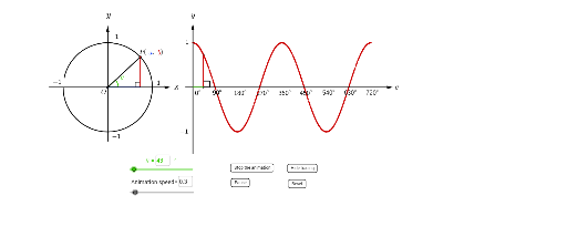
This example illustrates the geometric interpretation of the cosine function by dynamically rotating to show the relationship between angles and cosine values. Key mathematical concepts include trigonometry, vectors, coordinate geometry, and geometric transformations. Construction highlights the use of GeoGebra commands such as Segment, Circle, Intersect, Rotate, OrthogonalLine, Point, Ray, Angle, Textfield, Midpoint, Vector, If, and Polygon. Suitable for high school mathematics education, helping students understand the generation of trigonometric function graphs and the application of parametric equations.
GeoGebra Commands & Parameters
Segment(O, B_1) → h_1Circle(O, 3.141592653589793) → cIntersect(c, h_1) → D_1,Rotate(D_1, x(W), O) → A_{2}Intersect(xAxis, yAxis) → OriginSegment(Origin, O) → hIntersect(c, h) → D,OrthogonalLine(D, xAxis) → c_1Rotate(D, x(W), O) → AOrthogonalLine(A, xAxis) → gIntersect(g, xAxis) → BSegment(B, O) → kSegment(O, A) → bIntersect(b, k) → ESegment(A_{2}, O) → b_1Intersect(b_1, c_1) → FOrthogonalLine(Origin, xAxis) → dOrthogonalLine(Origin, d) → fPoint(xAxis) → GRay(Origin, G) → mAngle(D, O, A) → βTextfield(Θ) → inputBox1Segment(O, D) → aOrthogonalLine(A, a) → eSegment(A, B) → jSegment(W, Origin) → nSegment(X, W) → qSegment(W, Y) → sSegment(W, Z) → tAngle(A, B, O) → γSegment(F, D) → d_1Segment(F, A) → e_1Midpoint(q) → HMidpoint(s) → IMidpoint(t) → SSegment(B, O) → pPoint(yAxis) → PPoint(yAxis) → QVector(P, Q) → uPoint(u) → RPoint(xAxis) → TTextfield(speed) → inputBox2Angle(T, W, X) → δAngle(T, W, Y) → εVector(U, V) → zVector(A_1, B_1) → u_1Vector(A_1, B_1) → v_1Vector(C_1, T) → vVector(V, U) → z_1Segment(A_{2}, Y) → I_1Angle(D_1, O, A_{2}) → β_{1}OrthogonalLine(A_{2}, xAxis) → g_1Intersect(g_1, xAxis) → B_2Segment(A_{2}, B_2) → a_1Angle(A_{2}, B_2, O) → γ_1If(f_1 ≟ 1, true, false) → FAIf(f_1 ≟ 0, true, false) → FBPolygon(E_1, F_1, G_1, H_1) → poly1, e_2, f_2, g_2, h_2
AI Drawing Prompt Reference
Draw a dynamic illustration showing the geometric meaning of the cosine function, featuring a rotating circle and coordinate axes, with intersection points and line relationships demonstrating the correspondence between angles and cosine values, and label key angles and vectors to illustrate the generation process of trigonometric function graphs and parametric equations.
The prompt above was compiled from the original drawing commands and is for reference only.