Correlation Experimentation: Strong vs Weak Relationships

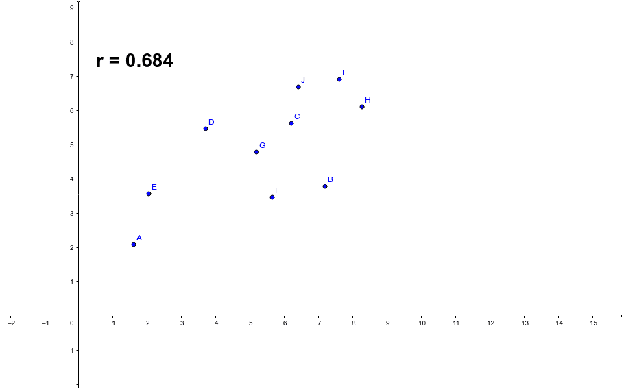
① This example demonstrates the visual difference between strong and weak correlations using scatter plots and a fitted line, allowing learners to grasp the meaning of correlation coefficients intuitively. ② The core mathematical concept is the Pearson product-moment correlation coefficient (PMCC), which quantifies the strength and direction of a linear relationship between two variables, ranging from -1 to 1, with values closer to ±1 indicating stronger correlation. ③ Construction details: The GeoGebra command PMCC is used to compute the correlation coefficient; points A through J serve as data samples; the variable r stores the coefficient value; and text1 dynamically displays the coefficient on the canvas, enabling real-time observation as data points are manipulated. ④ Suitable for high school or introductory college statistics, as well as math lab activities or inquiry-based learning, helping students distinguish between strong and weak, positive and negative correlations.