Continuous Chapman Layer (Algebraic)

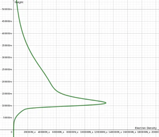
① This example demonstrates the algebraic modeling of a continuous Chapman layer in the ionosphere, showing the electron density distribution as a function of altitude with adjustable parameters and statistical characteristics. ② Core mathematical concepts include differential equations, definite integrals, frequency distributions, statistical measures, and inequalities, involving the Chapman function and layer structure parameters in atmospheric physics. ③ Construction highlights: Using GeoGebra commands such as Textfield, Segment, and Mirror, the applet provides interactive input boxes (InputBox1, InputBox3, InputBox6) and checkboxes (CasillaDeEntrada1-5), with objects like n_0, χ, z_{0E}, g_{Z0E}, M_E, T_e, N_{0E}, etc. Sliders and text dynamically adjust parameters, plotting curves for functions f, g, f_1, and using mirror tools to show symmetric layer structures. ④ Suitable for university-level physics or applied mathematics courses on ionospheric modeling, differential equation applications, and statistical distributions, as well as for research-based learning to explore how parameter changes affect layer shape.