
Constant Surfaces in Cartesian, Cylindrical, and Spherical Coordinate Systems
Loading the math board and drawing, please wait…
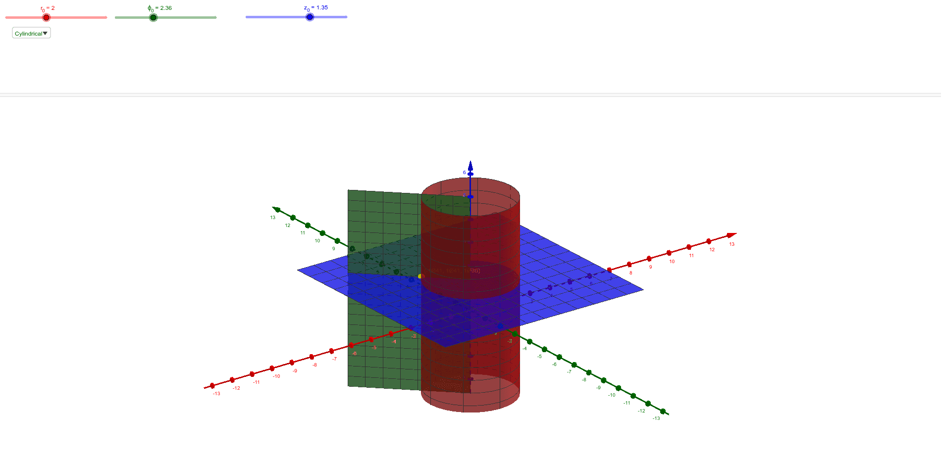
This example demonstrates the graphical representation of constant surfaces in Cartesian, cylindrical, and spherical coordinate systems. It involves core mathematical concepts such as coordinate transformations, 3D geometry, and constant surfaces. The construction uses GeoGebra commands like Surface, Sphere, Cone, and objects like System, si, x_0, y_0, z_0, etc. It is suitable for high school and above students to learn and understand geometric representations in multiple coordinate systems, useful for solid geometry and analytical geometry education.
GeoGebra Commands & Parameters
SelectedIndex(System) → siSurface(x_0, u, v, u, -5, 5, v, -5, 5) → X_0Surface(u, y_0, v, u, -5, 5, v, -5, 5) → Y_0Surface(u, v, z_0, u, -5, 5, v, -5, 5) → Z_0Surface((r_0 * cos(u)), (r_0 * sin(u)), v, u, 0, (2 * π), v, -5, 5) → R_0CSurface((u * cos(ϕ_0)), (u * sin(ϕ_0)), v, u, 0, 5, v, -5, 5) → T_0Sphere((0, 0, 0), r_0) → aCone((0, 0, (5 * cot(θ_0))), (0, 0, 0), 5) → b, b_2, b_3
AI Drawing Prompt Reference
Visualize constant surfaces in Cartesian, cylindrical, and spherical coordinate systems, highlighting core mathematical concepts like coordinate transformations, 3D geometry, and constant surfaces. Start by plotting the constant surfaces for each coordinate system, then add a sphere centered at the origin and a cone with its vertex at a point on the z-axis, ensuring the cone's base touches the sphere to demonstrate the relationship between different geometric shapes in 3D space.
The prompt above was compiled from the original drawing commands and is for reference only.