Concave Lens Ray Diagrams: Virtual Image and Diverging Light Paths

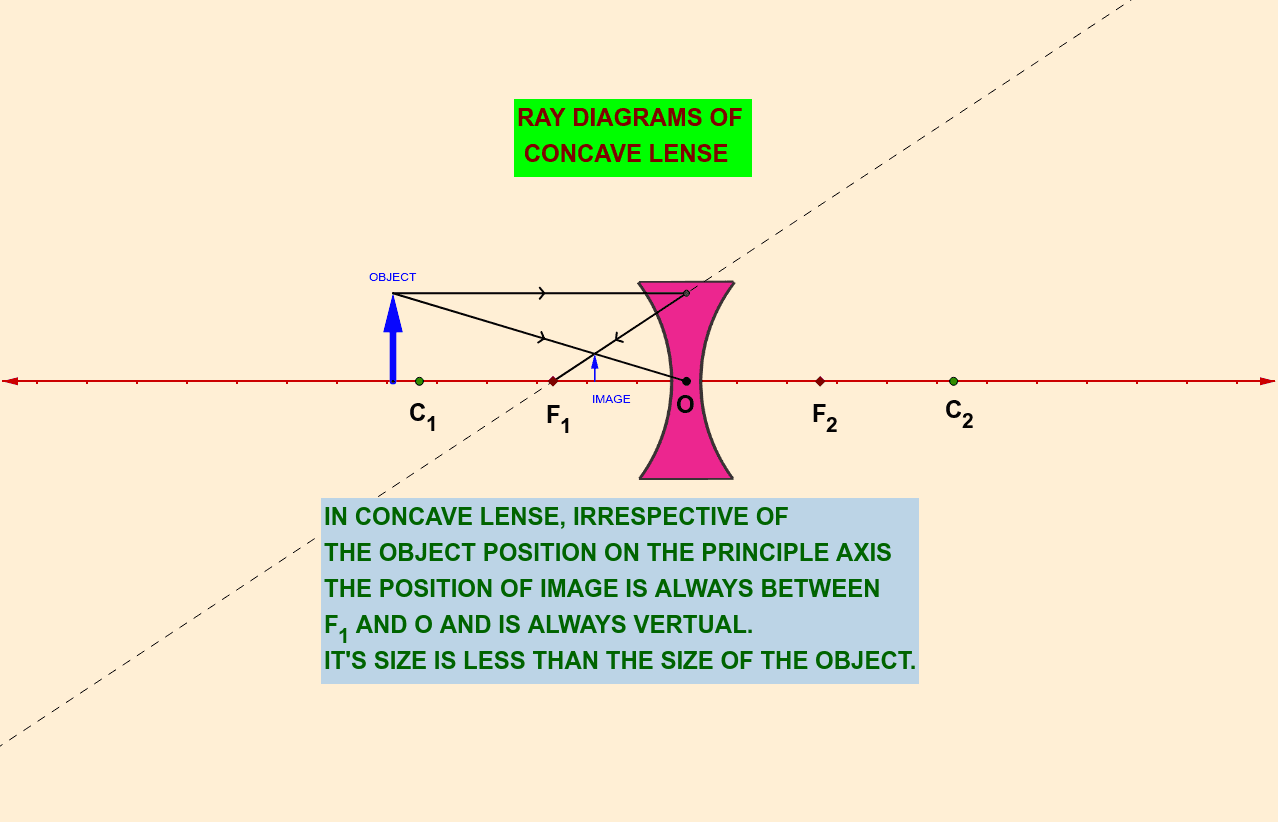
This GeoGebra example demonstrates how a concave lens refracts parallel rays and rays from a point source, clearly showing the formation of a virtual image through geometric construction. The core mathematical concepts include rectilinear propagation of light, geometric approximation of refraction, the relationship between virtual image position and focal length, and the use of similar triangles in ray path calculations. Construction highlights: using GeoGebra commands such as Point, OrthogonalLine, Vector, Line, Intersect, Segment, and Mirror, the model builds the principal axis, incident rays, and extended refracted rays, with intersections determining the virtual image location. Objects include pic1, A, B, a, C, OBJECT, b, D, c, E, d, e, f, g, F, G, h, H, IMAGE, I, I', E', and multiple text labels. Suitable for middle school physics optics lessons, geometric construction practice, and introductory university optics demonstrations, helping students understand the diverging nature of concave lenses and the rules of virtual image formation.