Compounding Interest in GeoGebra: Exponential Growth and Yield Curves

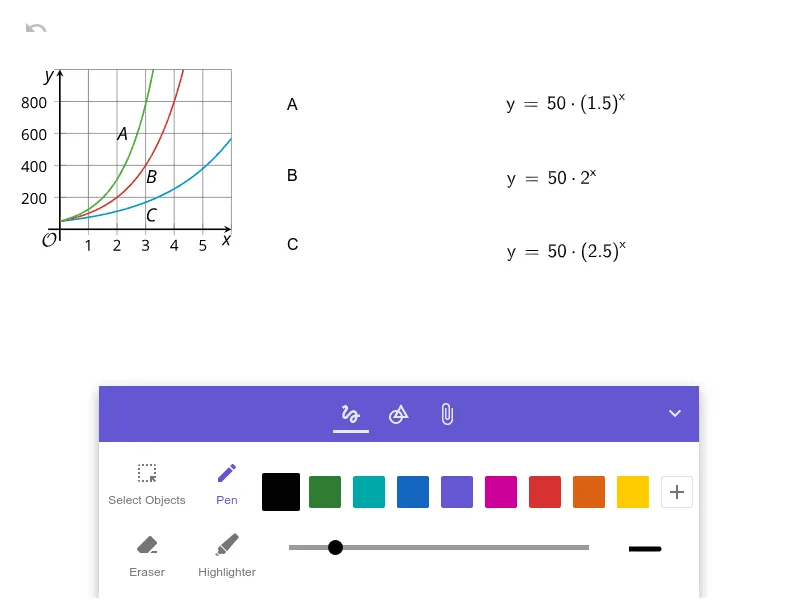
This example demonstrates how compounding interest grows over time: a principal accumulates by repeatedly adding interest at a fixed rate, producing an exponential-style growth pattern. The key concepts include the discrete compounding model, the relationship to exponential/power expressions, how time steps and the interest-rate parameter affect growth speed, and interpreting the results via graphing. For construction in GeoGebra, the typical workflow is to define a compounding-interest formula as a function object, introduce parameters (initial principal, rate, number of periods), and visualize the result using a function graph and/or plotted points across periods. Even though no GeoGebra command list is provided, the essential objects are usually function/graphing elements and (optionally) slider controls for interactive parameter changes. Suitable for late middle school through early university, especially for math modeling, quantitative reasoning, and finance-math visualization practice.