Composition of Linear Functions: Dynamic Graphing

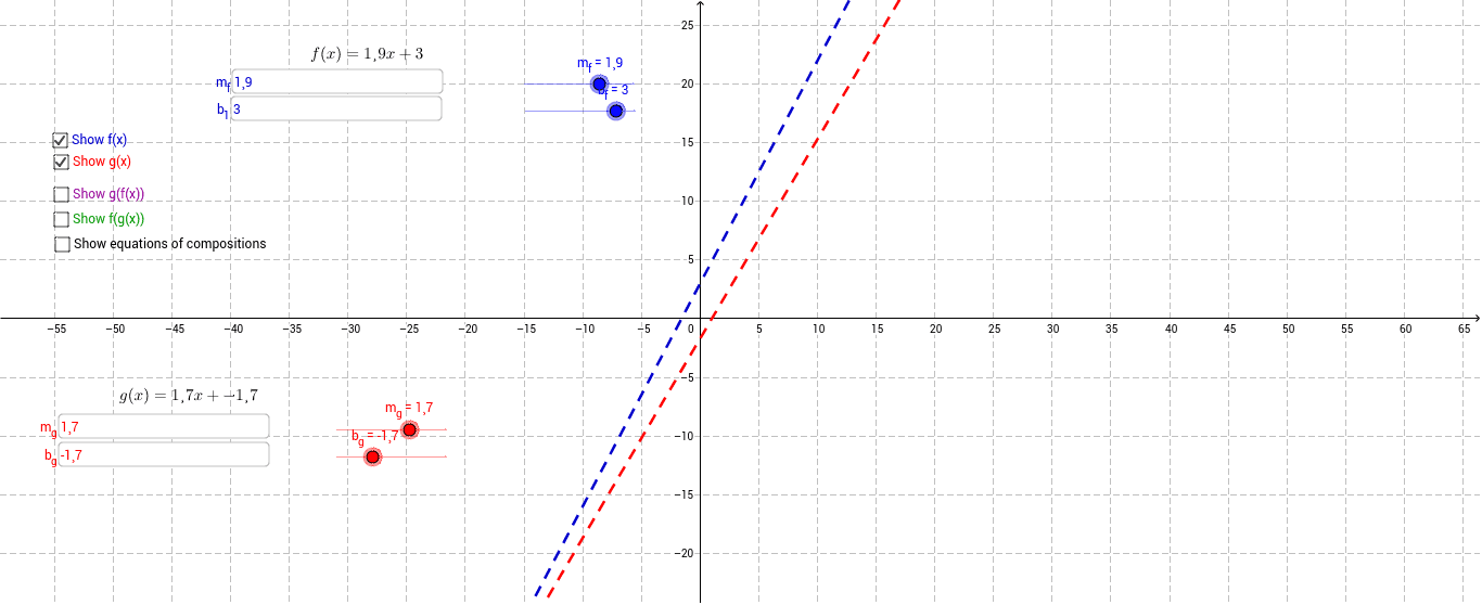
This interactive GeoGebra applet demonstrates the composition of two linear functions, allowing users to input coefficients and constants for f(x) = m_f·x + b_f and g(x) = m_g·x + b_g, then instantly view the graphs of the composite functions f(g(x)) and g(f(x)). Core mathematical concepts include linear functions, function composition, slope and y-intercept effects on line position and steepness, and the algebraic-geometric correspondence of composite linear mappings. Construction follows the GeoGebra command summary, using Textfield and inputBox input controls, parameter objects m_f, b_f, m_g, b_g, function objects f and g, auxiliary objects R, S, a, b, c, d, and text labels text1 through text4 and e. By adjusting linear coefficients, learners observe that composing two linear functions yields another linear function and explore how the resulting slope and intercept transform. Suitable for high school mathematics, introductory algebra, and function units, this resource supports classroom demonstrations, inquiry-based learning, and graphing visualization activities.