
Complex Mapping Diagrams for Quadratic Function and Solving Real Quadratic Equat
Loading the math board and drawing, please wait…
In collections
Mapping Diagrams to Visualize Complex Analysis
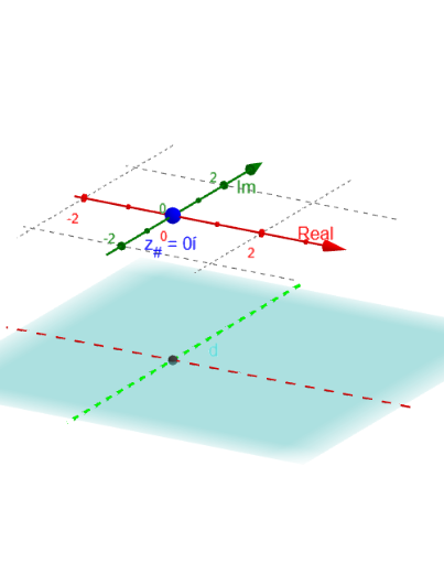
This example demonstrates the complex mapping diagram of a quadratic function and shows how to solve real quadratic equations using the complex mapping. Key math concepts include complex mapping, properties of quadratic functions, and solving real quadratic equations. GeoGebra commands used in construction are If, Sequence, Zip, Circle, Line, Vector, Point, Locus, Textfield, Intersect; objects include C_c, C_r, m, B_c, B_r, B, C, F, ht, z_#, f, fz_#, δ, n, M, t_*, z_*, showf, c, d, fz_*, fpt_*, O, ZX1, ZY1, Im_{axis}, Real_{axis}, fvec_*, fz1_#, vecf_#, A, Af, PtAf, fLoc, r2, u, r1, v, rlist, showroots. Suitable for high school mathematics education, to understand the relationship between complex mapping and solving real quadratic equations.
GeoGebra Commands & Parameters
If(m ≟ 1, B_c, B_r) → BIf(m ≟ 1, C_c, C_r) → CIf(m ≟ 1, F(z, B, C), F(z, B_r, C_r)) → fSequence(0, n) → MZip(((2 * pi) * k / n), k, M) → t_*Zip((δ * ℯ^((t * ί))) + z_#, t, t_*) → z_*Circle(z_#, δ) → cZip(f(z), z, z_*) → fz_*Zip((x(z), y(z), ht), z, fz_*) → fpt_*Line(O, ZY1) → Im_{axis}Line(O, ZX1) → Real_{axis}Zip(Vector[A, B], A, z_*, B, fpt_*) → fvec_*Vector(z_#, fz1_#) → vecf_#Point(c) → ALocus(PtAf, A) → fLocVector(r2, O) → uVector(r1, O) → vTextfield(F) → InputBox1Intersect(f_r, xAxis) → rr1, rr2
AI Drawing Prompt Reference
Create a diagram illustrating the complex mapping of a quadratic function, featuring real and imaginary axes, and the function's mapping trajectory in the complex plane. Start by plotting the origin and coordinate axes, then decide between B_c and B_r based on parameter m. Compute the function f's values and draw the mapping paths, showing vector changes and key points. Finally, use locus lines to represent the continuous mapping effect of the function.
The prompt above was compiled from the original drawing commands and is for reference only.