
Complex logarithm map (principal branch)
Loading the math board and drawing, please wait…
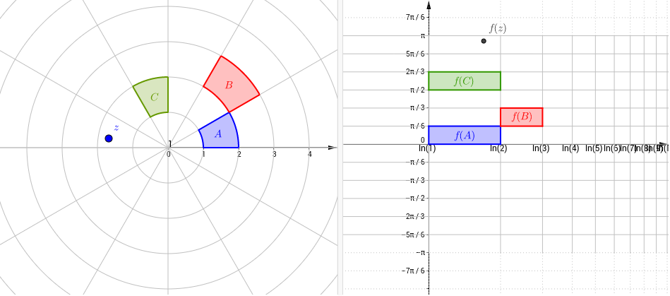
This example demonstrates the graph and properties of the complex logarithm map (principal branch). Key math concepts include complex numbers, logarithmic functions, and branch cuts. Construction highlights involve commands like Polygon, Point, Locus, and Sequence in GeoGebra. Suitable for high school and above students to understand the geometric meaning and branch characteristics of complex functions.
GeoGebra Commands & Parameters
Polygon(A, B, C, D) → regionA, a, b, c, dPolygon(E, F, G, H) → regionB, e, f, g, hPolygon(I, J, K, L) → regionC, i, j, k, lPoint(regionA) → z_1Locus(w_1, z_1) → fAPoint(regionB) → z_2Point(regionC) → z_3Locus(w_2, z_2) → fBLocus(w_3, z_3) → fCSequence(Line[(log(i / 100), 0), (log(i / 100), 1)], i, 1, 100) → GridXnSequence(Text["ln(" + (i) + ")", (log(i) - 0.1, -0.2)], i, 1, 1000) → AxisXlogSequence(Line[(0, (i * π / 6)), (1, (i * π / 6))], i, -5, 6) → GridYSequence(Line[(0, (i * π / 6)), (1, (i * π / 6))], i, 7, 20) → GridYupSequence(Line[(0, (i * π / 6)), (1, (i * π / 6))], i, -20, -6) → GridYdownSequence(Segment[(log(i), (-π)), (log(i), π)], i, 1, 1000) → GridXpSequence(Ray[(log(i), π), (log(i), (100 * π))], i, 1, 1000) → GridXpupSequence(Ray[(log(i), (-π)), (log(i), (-100 * π))], i, 1, 1000) → GridXpdown