
Cartesian and Polar Grapher
Loading the math board and drawing, please wait…
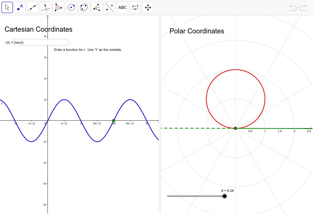
This example demonstrates how to sketch the graph of a polar equation by first plotting it in the Cartesian coordinate system for better visualization. Key math concepts include polar and Cartesian coordinate conversion, function graphing, and trigonometric applications. Construction highlights involve using GeoGebra commands like CurveCartesian for Cartesian curves, Ray and Segment for rays and line segments, and Textfield for text annotations, with parameters θ, r, a, b, c. Suitable for high school mathematics education to understand the relationship between polar equations and Cartesian coordinates, and the methods of function graphing.
GeoGebra Commands & Parameters
CurveCartesian((r(t) * cos(t)), (r(t) * sin(t)), t, 0, θ) → aRay((0, 0), (cos(θ), sin(θ))) → posRayRay((0, 0), ((-cos(θ)), (-sin(θ)))) → negRaySegment(onCart, (x(onCart), 0)) → bSegment(onCart, (x(onCart), 0)) → cTextfield(r) → inputBox1
AI Drawing Prompt Reference
Sketch the graph of a polar equation in the Cartesian coordinate system first, then draw the positive and negative rays at angle θ. Finally, draw two segments from a point on the curve to the positive and negative x-axis directions.
The prompt above was compiled from the original drawing commands and is for reference only.