
Calculus & Trigonometry Integration Example
Loading the math board and drawing, please wait…
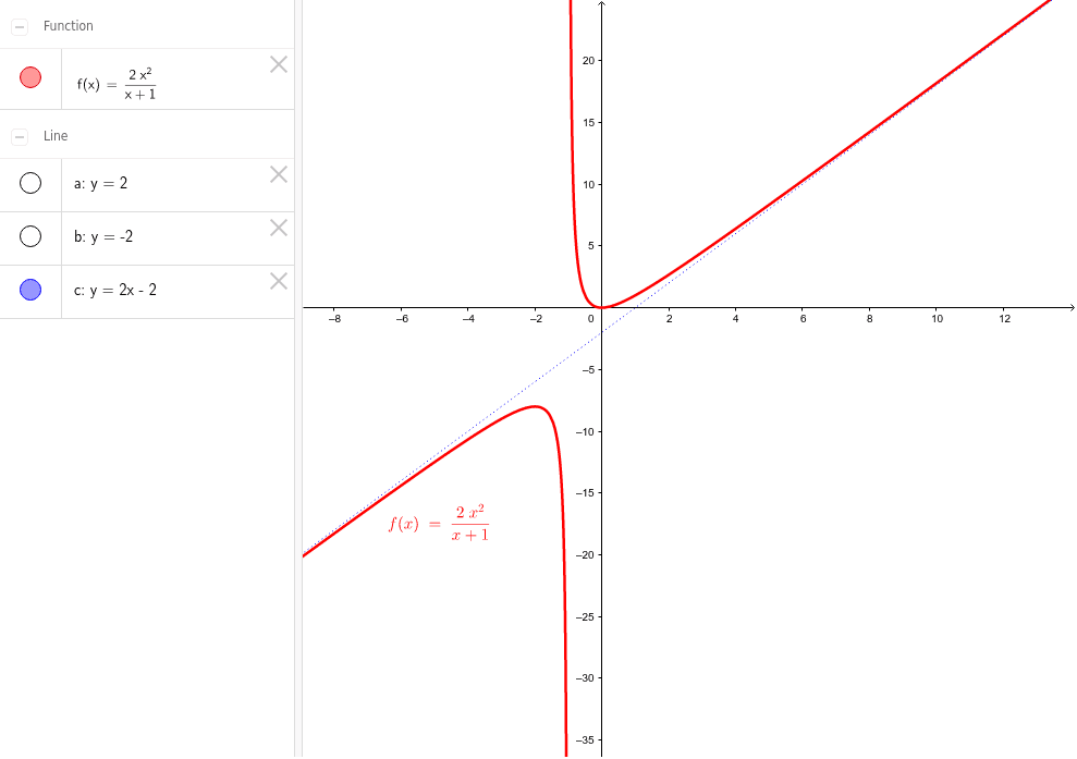
This example demonstrates the integration of calculus, limits, trigonometric functions, and standard deviation in geometric transformations, showcasing dynamic intersections between function graphs and circles. Key math concepts include limits in calculus, properties of trigonometric functions, standard deviation calculation, and geometric transformations. Construction highlights involve GeoGebra objects: f for the function, and a, b, c as parameters controlling function shape and transformation. Suitable for high school and above students studying calculus, trigonometry, and geometric transformations to understand function optimization and geometric properties.
GeoGebra Commands & Parameters
f(x) = ((2 * x^(2))) / (x + 1)Line a(0.0, 1.0, -2.0)Line b(0.0, 1.0, 2.0)Line c(-2.0, 1.0, 2.0)
AI Drawing Prompt Reference
Draw a function graph where the function is 2x squared divided by x plus 1, and plot three lines: one extending from (0,1) to the left until (-2,1), another from (0,1) to the right until (2,1), and the last from (-2,1) to the right until (2,1), showing dynamic intersections with the function, demonstrating calculus limits, trigonometric properties, standard deviation calculation, and geometric transformations.
The prompt above was compiled from the original drawing commands and is for reference only.