
Bivariate Normal Distribution by Peter Sassman
Loading the math board and drawing, please wait…
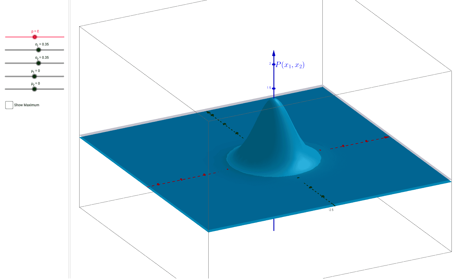
This example demonstrates the joint probability density function of a bivariate normal distribution, including its contour plot. Key mathematical concepts involved are normal distribution, random variables, mean vector, covariance matrix, and probability density function. The construction leverages GeoGebra commands and objects like p, σ_1, σ_2, a, Coeff, μ_1, μ_2, Denom, d, b, Maximum, text1, Max, text2, text3, text4 to visualize how changes in parameters affect the distribution shape. Suitable for high school students and researchers in mathematics and statistics studying probability distributions and parameter influences.
GeoGebra Commands & Parameters
Numeric p(0.0)Numeric σ_1(0.35)Numeric σ_2(0.35)a:1 / ((2 * π))1 / (((((2 * π) * σ_1) * σ_2) * sqrt(1 - p^(2))))Numeric μ_1(0.0)Numeric μ_2(0.0)-1 / ((2 * (1 - p^(2))))d(x, y) = (Coeff * ℯ^((Denom * ((x - μ_1)^(2) / σ_1^(2) - (((2 * p) * (x - μ_1)) * (y - μ_2) / ((σ_1 * σ_2))) + (y - μ_2)^(2) / σ_2^(2)))))b:z = 0.05(μ_1, μ_2, Coeff)Boolean Max(false)