
Binomial Probability - PDF and CDF
Loading the math board and drawing, please wait…
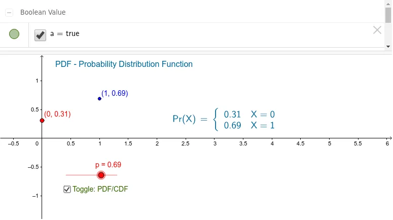
This example demonstrates the probability density function (PDF) and cumulative distribution function (CDF) of the binomial distribution, showing how they change with parameters. Key math concepts include probability & statistics, distribution functions, and parameter effects. GeoGebra commands used: p (probability), q (complement), A (text), B (text), pdftxt (text), O (point), C (point), cdftxt (text), a (value), b (value), F (function), D (function), cdfFtxt (text), pdfftxt (text). Suitable for high school and above students learning distribution function properties in probability statistics.
GeoGebra Commands & Parameters
Numeric p(0.69)1 - p(0, q)(1, p)Point O(0.0, 0.0)A + BBoolean a(true)¬aF(x) = If[x < 0, 0,If[x < 1, q,1]](1, q)
AI Drawing Prompt Reference
Draw a graph illustrating the probability density function (PDF) and cumulative distribution function (CDF) of a binomial distribution with p=0.69. Include two points at (0,0) and (1,q), where q is the complement of p. Define a function F(x) that is 0 for x<0, q for 0<x<1, and 1 otherwise. Also, plot a line segment from (0,0) to (1,q) and label the values of p, q, and the definitions of the two functions to show how parameters affect the distribution functions.
The prompt above was compiled from the original drawing commands and is for reference only.