
Binomial Distribution with Probability over an Interval
Loading the math board and drawing, please wait…
In collections
UNSW MATH1131/1231 Algebra material
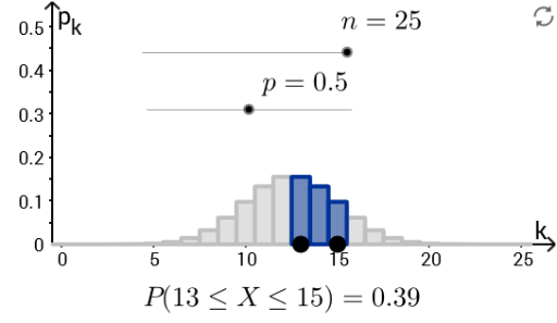
This GeoGebra example visualizes the binomial distribution over a specified probability interval. It demonstrates how to compute and plot cumulative probabilities, interval-based distribution characteristics, and key statistical measures such as mean (μ) and standard deviation (σ). Core concepts include binomial distribution, probability intervals, variance, expected value, and cumulative frequency. Construction uses GeoGebra commands like Join, Sequence, and Point, along with objects representing trial count (n), success probability (p), failure probability (q), distribution functions (f, F), and statistical summaries (μ, σ). Sliders and dynamic objects allow interactive exploration of how changing n and p affects the distribution shape and interval probabilities. Suitable for high school and early college statistics courses, it supports teaching probability theory, distribution visualization, and interval-based inference concepts.
GeoGebra Commands & Parameters
Join({Sequence[((n! / ((i! * (n - i)!)) * p^(i)) * q^(n - i)), i, 0, n], Sequence[0, k, 0, 30]}) → fSequence(Sum[Sequence[((n! / i! / (n - i)! * p^(i)) * q^(n - i)), i, 0, k]], k, 0, n) → FSequence(Polygon[(i - d, 0), (i + d, 0), (i + d, Element[f, i + 1]), (i - d, Element[f, i + 1])], i, 0, n, 1) → PlotfSequence(Polygon[(i - d, 0), (i + d, 0), (i + d, Element[F, i + 1]), (i - d, Element[F, i + 1])], i, 0, n, 1) → PlotFSequence((k, 0), k, 0, n_max) → list1Point(list1) → APoint(list1) → BSequence(Polygon[(i - d, 0), (i + d, 0), (i + d, Element[f, i + 1]), (i - d, Element[f, i + 1])], i, Min[x(A), x(B)], Min[Max[x(A), x(B)], n], 1) → list2
AI Drawing Prompt Reference
Draw a binomial distribution visualization over a probability interval. The horizontal axis represents the number of successes, and the vertical axis represents probability. Use a series of rectangles with fixed width and height equal to the probability of each success count. Overlay another set of rectangles for cumulative probabilities, showing the sum from zero to each count. Place draggable points on the horizontal axis to select the left and right boundaries of the interval. When dragging, highlight the rectangles within the interval and automatically compute the cumulative probability for that range. Include step-like curves for both the probability mass function and the cumulative distribution function. Provide sliders to adjust the number of trials and success probability, dynamically updating the shape and interval probabilities.
The prompt above was compiled from the original drawing commands and is for reference only.