
Binomial Distribution with Normal and Poisson Approximation
Loading the math board and drawing, please wait…
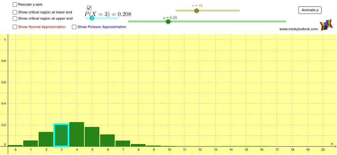
① This applet dynamically visualizes the binomial distribution and overlays normal and Poisson approximation curves, allowing users to observe how well these continuous approximations fit the discrete distribution under varying parameters. ② Core mathematical concepts include binomial distribution, normal distribution, Poisson distribution, expected value μ, standard deviation σ, probability mass function, probability density function, and the central limit theorem as applied to discrete approximations. ③ Construction highlights: using GeoGebra commands such as Sequence to generate probability points, Polygon for the bar chart, Line for the normal curve, Sum and Integral for cumulative probabilities, sliders to control n and p, If and Slider objects for interactivity, plus critical value sequences and play buttons for animation. ④ Suitable for high school to undergraduate probability and statistics courses, ideal for classroom demonstrations and self-guided exploration of how the binomial distribution changes with n and p, and when normal or Poisson approximations are appropriate.
GeoGebra Commands & Parameters
Sequence(Polygon[(i - 0.475, 0), (i - 0.475, ((Binomial[n, i] * p^(i)) * (1 - p)^(n - i))), (i + 0.45, ((Binomial[n, i] * p^(i)) * (1 - p)^(n - i))), (i + 0.45, 0)], i, 0, n) → list1If(b, Max[list1] / 0.925, 1) → aIf(b, 1, 0) → cPolygon((-2, 1.05), (-2, 1.6), (103, 1.6), (103, 1.05)) → poly1, f, g, h, iSequence(Polygon[(i - 0.475, 0), (i - 0.475, ((Binomial[n, i] * p^(i)) * (1 - p)^(n - i))), (i + 0.45, ((Binomial[n, i] * p^(i)) * (1 - p)^(n - i))), (i + 0.45, 0)], i, 0, criticallow) → list2Sequence(Polygon[(i - 0.475, 0), (i - 0.475, ((Binomial[n, i] * p^(i)) * (1 - p)^(n - i))), (i + 0.45, ((Binomial[n, i] * p^(i)) * (1 - p)^(n - i))), (i + 0.45, 0)], i, criticalhigh, n) → list3Line(A, B) → kIf(n ≤ 20, 20, n) → xmaxSequence(Polygon[(i - 0.475, 0), (i - 0.475, (ℯ^(((-n) * p)) * ((n * p))^(i) / i!)), (i + 0.45, (ℯ^(((-n) * p)) * ((n * p))^(i) / i!)), (i + 0.45, 0)], i, 0, n) → list4Sequence(((Binomial[n, i] * p^(i)) * (1 - p)^(n - i)), i, 0, criticallow) → criticallowsequenceSum(criticallowsequence) → criticallowvalueSequence(((Binomial[n, i] * p^(i)) * (1 - p)^(n - i)), i, criticalhigh, n) → criticalhighsequenceSum(criticalhighsequence) → criticalhighvalueIf(d, criticallow + 1, 0) → criticalhighsliderminPolygon((m - 0.475, 0), (m - 0.475, ((Binomial[n, m] * p^(m)) * (1 - p)^(n - m))), (m + 0.45, ((Binomial[n, m] * p^(m)) * (1 - p)^(n - m))), (m + 0.45, 0)) → poly2, r, s, t, a_1Integral(q, -50, criticallow + 0.5) → criticallownormalIntegral(q, criticalhigh - 0.5, n + 50) → criticalhighnormal
AI Drawing Prompt Reference
Draw a bar chart of the binomial probability mass function with the number of trials on the x-axis and probability on the y-axis. Use sliders to adjust the number of trials and success probability. Overlay a normal distribution curve and a Poisson distribution curve for approximation comparison. Use distinct colors or transparency to differentiate the binomial bars, normal curve, and Poisson curve. Shade the cumulative probability regions for the left and right tails, highlighting the critical value ranges. Add a highlighted bar to mark the current critical value position. Include a legend and axis labels for clarity, allowing observation of how well the continuous approximations fit the discrete distribution.
The prompt above was compiled from the original drawing commands and is for reference only.