
Binomial Distribution with Normal and Poisson Approximation by gesges
Loading the math board and drawing, please wait…
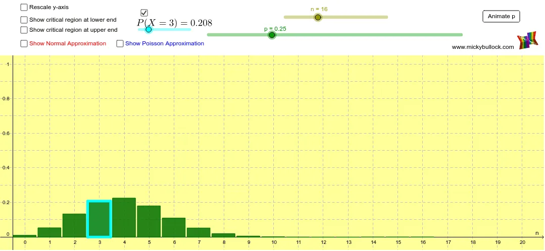
This applet visualizes the Binomial Distribution and its Normal and Poisson approximations. By adjusting parameters n and p, you can observe changes in the distribution curves. It uses GeoGebra commands such as Sequence, If, Polygon, Line, Sum, and Integral for construction. Suitable for high school and above students or teachers for probability and statistics education.
GeoGebra Commands & Parameters
Sequence(Polygon[(i - 0.475, 0), (i - 0.475, ((Binomial[n, i] * p^(i)) * (1 - p)^(n - i))), (i + 0.45, ((Binomial[n, i] * p^(i)) * (1 - p)^(n - i))), (i + 0.45, 0)], i, 0, n) → list1If(b, Max[list1] / 0.925, 1) → aIf(b, 1, 0) → cPolygon((-2, 1.05), (-2, 1.6), (103, 1.6), (103, 1.05)) → poly1, f, g, h, iSequence(Polygon[(i - 0.475, 0), (i - 0.475, ((Binomial[n, i] * p^(i)) * (1 - p)^(n - i))), (i + 0.45, ((Binomial[n, i] * p^(i)) * (1 - p)^(n - i))), (i + 0.45, 0)], i, 0, criticallow) → list2Sequence(Polygon[(i - 0.475, 0), (i - 0.475, ((Binomial[n, i] * p^(i)) * (1 - p)^(n - i))), (i + 0.45, ((Binomial[n, i] * p^(i)) * (1 - p)^(n - i))), (i + 0.45, 0)], i, criticalhigh, n) → list3Line(A, B) → kIf(n ≤ 20, 20, n) → xmaxSequence(Polygon[(i - 0.475, 0), (i - 0.475, (ℯ^(((-n) * p)) * ((n * p))^(i) / i!)), (i + 0.45, (ℯ^(((-n) * p)) * ((n * p))^(i) / i!)), (i + 0.45, 0)], i, 0, n) → list4Sequence(((Binomial[n, i] * p^(i)) * (1 - p)^(n - i)), i, 0, criticallow) → criticallowsequenceSum(criticallowsequence) → criticallowvalueSequence(((Binomial[n, i] * p^(i)) * (1 - p)^(n - i)), i, criticalhigh, n) → criticalhighsequenceSum(criticalhighsequence) → criticalhighvalueIf(d, criticallow + 1, 0) → criticalhighsliderminPolygon((m - 0.475, 0), (m - 0.475, ((Binomial[n, m] * p^(m)) * (1 - p)^(n - m))), (m + 0.45, ((Binomial[n, m] * p^(m)) * (1 - p)^(n - m))), (m + 0.45, 0)) → poly2, r, s, t, a_1Integral(q, -50, criticallow + 0.5) → criticallownormalIntegral(q, criticalhigh - 0.5, n + 50) → criticalhighnormal
AI Drawing Prompt Reference
Draw the binomial distribution and its normal and Poisson approximations. First, plot the binomial distribution bars based on parameters n and p. Then, adjust n and p to observe changes in the distribution curves. Next, shade the area for the normal approximation and mark its upper and lower bounds. Finally, plot the Poisson approximation bars and adjust n and p to observe changes.
The prompt above was compiled from the original drawing commands and is for reference only.