Binomial Distribution vs. Normal Approximation

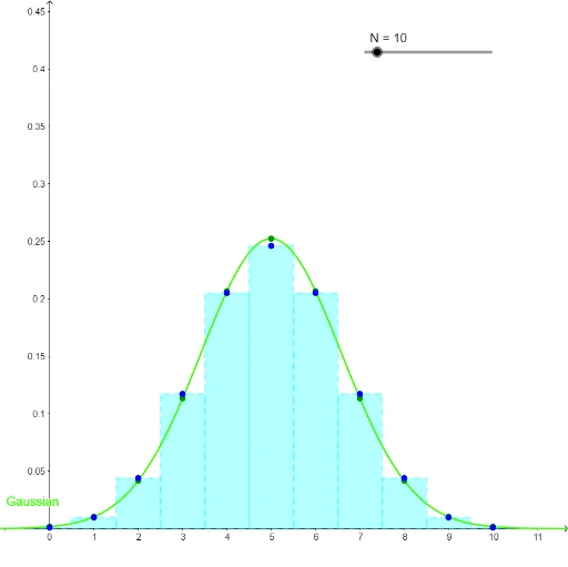
This GeoGebra example visualizes the normal approximation to the binomial distribution. As the number of independent trials increases, the binomial probability mass function gradually approaches the continuous normal probability density function. The demonstration illustrates the relationship between discrete probability distributions and their continuous limits, grounded in the Central Limit Theorem. Key mathematical concepts include binomial distribution, normal approximation, probability mass versus density functions, and limit theorems. The construction employs GeoGebra commands Sequence and Sum to generate trial data sequences, alongside discrete Gaussian function Gaussian_{discrete} and continuous Gaussian function Gaussian for overlay plotting. It is suitable for high school statistics units and introductory college probability courses, helping learners develop intuition about when and why the normal approximation is valid and effective.