Asymptotes for Rational Functions: Vertical, Horizontal, and Oblique

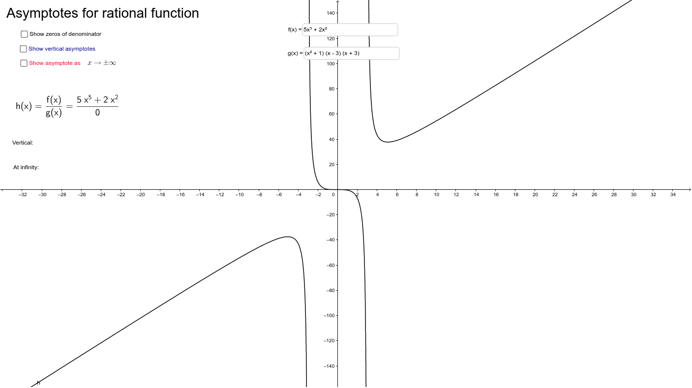
This GeoGebra example dynamically illustrates the vertical, horizontal, and oblique asymptotes of a rational function, showing how the graph approaches these lines as x tends to infinity or near discontinuities. Core mathematical concepts include rational functions, polynomial division, asymptote definitions (vertical asymptotes at denominator zeros; horizontal/oblique asymptotes determined by degree comparison), and limit behavior. Construction highlights: uses the Div command for polynomial division to obtain the quotient (oblique asymptote equation), Coefficients and Degree to extract polynomial data, Derivative for analysis, Point and Line to draw asymptote lines, Textfield and text objects for dynamic equations and explanations, Intersection for key points, and sliders (a, b, c, d) to adjust function parameters and observe changes in real time. Suitable for senior high school or pre-calculus/calculus courses, this tool helps students understand rational function graphs and algebraic methods for finding asymptotes, and serves as an interactive classroom demonstration or self-study resource.