
Area Under a Curve: Interactive Integral and Geometric Transformations
Loading the math board and drawing, please wait…
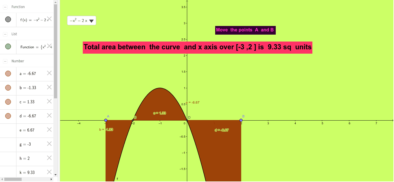
This GeoGebra example demonstrates how to dynamically compute the area between a function curve and the x-axis, visually illustrating the geometric meaning of definite integrals. Core mathematical concepts include definite integrals, area calculation, function graphing, and geometric transformations (such as similarity) affecting area. Construction highlights: using Function to define f, Point and Intersect to set interval endpoints A and B, Integral to generate the shaded region, and SelectedElement, Slider, Tangent Line, and Similarity Transformation to explore dynamic parameter changes and their effects. Suitable for high school to undergraduate calculus instruction, this resource helps students connect integrals with area, understand transformation invariance, and investigate how similarity scaling alters area values.
GeoGebra Commands & Parameters
SelectedElement(Function) → fPoint(xAxis) → APoint(xAxis) → BIntegral(f, x(A), x(B)) → aIntersect(f, xAxis) → C, DIntegral(f, x(A), x(C)) → bIntegral(f, x(C), x(D)) → cIntegral(f, x(D), x(B)) → d
AI Drawing Prompt Reference
Draw a function curve and shade the region between the curve and the x-axis to represent a definite integral. Place two movable points on the x-axis as the left and right endpoints of the integration interval, with vertical boundaries from the curve to the axis. Mark all intersection points of the curve with the x-axis, and divide the interval into segments at these points, shading each segment with a different intensity. Add a slider to dynamically adjust a parameter (such as a scaling factor), and display a tangent line to show how the shaded area changes under geometric transformations like similarity.
The prompt above was compiled from the original drawing commands and is for reference only.