
Area of a Circle: From Sectors to Integral
Loading the math board and drawing, please wait…
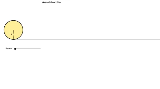
This GeoGebra example dynamically demonstrates the derivation of the circle area formula A=πr² by partitioning the circle into sectors and rearranging them to approximate a rectangle, while also connecting to the concept of definite integrals. Core mathematical concepts include circle area, sectors, arc length, rotation, congruence, and integration. The construction uses a slider to control the number of divisions n, Sequence to generate equally spaced points, Rotate to reposition sectors, Sector and Arc to create sector regions, CurveCartesian to draw boundary curves, Circle and Ray for auxiliary construction, Midpoint and Intersect to compute key points, and multiple text objects to display dynamic area values and formulas. Suitable for middle school geometry, introductory calculus, and math lab activities, helping learners transition from visual intuition to rigorous integral-based reasoning.
GeoGebra Commands & Parameters
Segment(E, (x(E) + 2, y(E))) → aPoint(a) → FMin(x(F) - x(E), 1) → kPoint(yAxis) → OSequence(If[k < 1, (x(O) + ((l * sin((i * φ))) * cos((i * φ)) / sin(φ)), y(O) + ((l * sin((i * φ))) * sin((i * φ)) / sin(φ))), (x(O) + (l * i), y(O))], i, 0, (2 * n)) → list2Sequence((x(O) + sin((i * θ)), y(O) + 1 - cos((i * θ))), i, 0, (2 * n)) → list1Max(x(F) - x(E) - 1, 0) → k'Rotate((x(O) + 0, y(O) + 1), ((-k) * θ / 2), O) → ARotate(O, ((-k) * θ / 2), O) → O'Rotate(Element[list1, 1], ((-k) * θ / 2), O) → BSector(Rotate[Circle[(x(O) + 0, y(O) + 1), O], ((-k) * θ / 2), O], Rotate[O, ((-k) * θ / 2), O], Rotate[Element[list1, 1], ((-k) * θ / 2), O]) → cRotate((x(O) + 0, y(O) + 1), ((-k) * θ / 2), O) → CRotate(O, ((-k) * θ / 2), O) → O'_1Rotate(Element[list1, 1], ((-k) * θ / 2), O) → DArc(Rotate[Circle[(x(O) + 0, y(O) + 1), O], ((-k) * θ / 2), O], O'_1, D) → dCurveCartesian(t - sin(t), 1 - cos(t), t, 0, 6.28319) → bCircle((0, 1), 1) → hRay((0, 0), (1, 0)) → iPoint(Segment[(0, 1), (6.28319, 1)]) → HSegment(H, (x(H), 0)) → jMidpoint(j) → IMidpoint(a) → JCircle(L, 1 / (1 - m)) → pCircle((0, 0), 1 / (1 - m)) → qIntersect(p, q, 1) → MIntersect(p, q, 2) → NCircle((0, 1), 1) → c_1Segment((0, 0), (6.283185307179586, 0)) → eSegment(G, (x(G), y(G) - 1)) → rSequence(Sector[Rotate[Translate[Circle[(x(O) + 0, y(O) + 1), Element[list1, i]], Vector[Element[list1, i], Element[list2, i]]], (((-((2 * i) - 1)) * k) * θ / 2), Element[list2, i]], Rotate[Translate[Element[list1, i], Vector[Element[list1, i], Element[list2, i]]], (((-((2 * i) - 1)) * k) * θ / 2), Element[list2, i]], Rotate[Translate[Element[list1, i + 1], Vector[Element[list1, i], Element[list2, i]]], (((-((2 * i) - 1)) * k) * θ / 2), Element[list2, i]]], i, 1, n) → list3Sequence(Sector[Rotate[Rotate[Translate[Circle[(x(O) + 0, y(O) + 1), Element[list1, i]], Vector[Element[list1, i], Element[list2, i]]], (((-((2 * i) - 1)) * k) * θ / 2), Element[list2, i]], (180° * k'), (x(O) + (n * l) - sin(θ / 2) / 2, y(O) + cos(θ / 2) / 2)], Rotate[Rotate[Translate[Element[list1, i], Vector[Element[list1, i], Element[list2, i]]], (((-((2 * i) - 1)) * k) * θ / 2), Element[list2, i]], (180° * k'), (x(O) + (n * l) - sin(θ / 2) / 2, y(O) + cos(θ / 2) / 2)], Rotate[Rotate[Translate[Element[list1, i + 1], Vector[Element[list1, i], Element[list2, i]]], (((-((2 * i) - 1)) * k) * θ / 2), Element[list2, i]], (180° * k'), (x(O) + (n * l) - sin(θ / 2) / 2, y(O) + cos(θ / 2) / 2)]], i, n + 1, (2 * n)) → list4CircleArc((0, 1 / (1 - m)), O, L) → sSegment(Q, R) → g
AI Drawing Prompt Reference
Draw a dynamic diagram illustrating the area formula of a circle. A circle is divided into many sectors, with a slider controlling the number of divisions. When the number is small, sectors remain in a circular arc; as it increases, sectors are translated and rotated to rearrange into an approximate rectangle. One side of the rectangle equals the radius, the other equals half the circumference (πr). Include a cycloid curve as a boundary reference, along with auxiliary circles, rays, and segments. Mark key points and midpoints, and display dynamic area values and formulas to show the transition from sectors to integral-based area calculation.
The prompt above was compiled from the original drawing commands and is for reference only.