
Arbitrary Cone
Loading the math board and drawing, please wait…
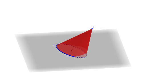
This example demonstrates the construction of an arbitrary cone. It involves basic concepts of a cone such as base radius, height, and slant height. Using GeoGebra commands like Intersect, PointIn, Distance, Angle, and Surface, the shape of the cone can be dynamically adjusted. Suitable for high school geometry courses.
GeoGebra Commands & Parameters
Intersect(zAxis, xAxis) → APointIn(Plane[xAxis, zAxis]) → BDistance(A, B) → rAngle((1, 0, 0), A, B) → aSurface((((r * cos(u)) * cos(a)) * v) + ((1 - v) * x(S)), ((r * sin(u)) * v) + ((1 - v) * y(S)), ((((sgn(z(B)) * r) * cos(u)) * sin(a)) * v) + ((1 - v) * z(S)), u, 0, (2 * π), v, 0, 1) → bCurveCartesian(((r * cos(u)) * cos(a)), (r * sin(u)), (((sgn(z(B)) * r) * cos(u)) * sin(a)), u, 0, (2 * π)) → c
AI Drawing Prompt Reference
Draw an arbitrary cone by first defining its axis and base center point. Then, use the base radius and the angle between the axis and the base center to define the cone's shape. Dynamically adjust the cone's size using the base radius and angle, and finally depict the cone's surface through the intersection of a plane and a surface.
The prompt above was compiled from the original drawing commands and is for reference only.