
A Geometric Visual Proof of Pythagorean Theorem
Loading the math board and drawing, please wait…
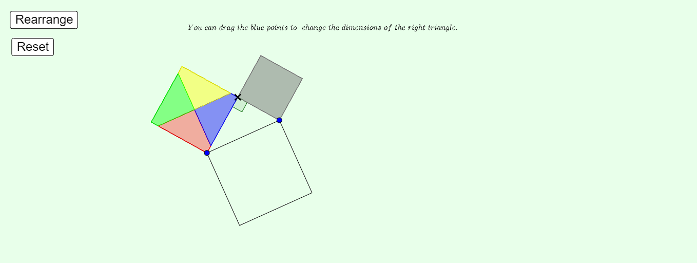
This example uses an interactive geometric construction to visually demonstrate the Pythagorean Theorem by decomposing and reassembling a right triangle, making the relationship a^2 + b^2 = c^2 visually apparent through area/length equivalence. It centers on concepts of right triangles, the Pythagorean Theorem, and proof-by-geometry via precise construction and transformation. Construction approach: it builds the main figures with GeoGebra commands such as Segment (segments), Point (points), Line/Ray (lines/rays), and Angle (angles), then uses Polygon to outline regions used in the argument. Circles and auxiliary geometry are created with Circle and Semicircle, while Intersect helps locate key intersection points. Midpoint supports midpoint-based steps, and Vector with Translate plus Dilate provides controlled transformations to generate corresponding parts that match the theorem’s required correspondence. The construction culminates in objects that encode the equality (e.g., equals) that expresses the final relationship. Suitable for middle and high school geometry lessons, interactive proof practice, and self-study demonstrations.
GeoGebra Commands & Parameters
Segment(A, B) → cSemicircle(A, B) → c_2Point(c_2) → CSegment(B, C) → bSegment(C, A) → aAngle(A, C, B) → αPolygon(C, B, 4) → small_1, e, f, g, h, D, EPolygon(A, C, 4) → poly2, i, j, k, l, F, GPolygon(B, A, 4) → poly3, m, n, p, q, H, IMidpoint(D, C) → JMidpoint(F, A) → LMidpoint(I, A) → KVector(J, K) → vTranslate(D, v) → D'Translate(C, v) → C'Translate(E, v) → E'Translate(B, v) → B'Ray(B', D') → rRay(D', E') → sRay(E', C') → tRay(C', B') → a_1Segment(I, H) → b_1Segment(H, A) → c_1Segment(B, I) → d_1Intersect(a_1, b_1) → MIntersect(t, c_1) → NIntersect(r, d_1) → OIntersect(c, s) → PDilate(D', 1 - equals / 100, A) → D''Circle(G, Segment[B', M]) → e_1Segment(F, G) → g_1Segment(A, G) → h_1Segment(C, F) → i_1Intersect(e_1, h_1, 1) → QCircle(A, Segment[G, Q]) → k_1Circle(C, Segment[G, Q]) → q_1Circle(F, Segment[G, Q]) → r_1Intersect(e_1, g_1, 1) → RIntersect(r_1, g_1, 1) → SIntersect(q_1, a, 1) → TIntersect(k_1, a, 1) → UIntersect(k_1, h_1, 1) → VIntersect(q_1, i_1, 1) → WIntersect(r_1, i_1, 1) → ZPolygon(F, W, L, S) → yellow_1, y1A, y1D, y1B, y1CPolygon(S, L, Q, G) → green_1, g1B, g1C, g1D, g1APolygon(L, U, A, Q) → red_1, r1B, r1C, r1D, r1APolygon(U, L, W, C) → blue_1, b1D, b1A, b1B, b1CDilate(D', equals / 100, A) → D''_1Vector(A, D''_1) → v_1Translate(L, v_1) → L'Translate(U, v_1) → U'Translate(A, v_1) → A'Translate(Q, v_1) → Q'Polygon(L', U', A', Q') → red_1', r1B', r1C', r1D', r1A'Dilate(P, equals / 100, W) → P'Vector(W, P') → j_1Translate(U, j_1) → U'_1Translate(L, j_1) → L'_1Translate(W, j_1) → W'Translate(C, j_1) → C'_1Polygon(U'_1, L'_1, W', C'_1) → blue_1', b1D', b1A', b1B', b1C'Dilate(K, equals / 100, J) → K'Vector(J, K') → m_1Translate(small_1, m_1) → small_1'Dilate(H, equals / 100, L) → H'Vector(L, H') → n_1Translate(F, n_1) → F'Translate(W, n_1) → W'_1Translate(L, n_1) → L'_2Translate(S, n_1) → S'Polygon(F', W'_1, L'_2, S') → yellow_1', y1A', y1D_1, y1B_1, y1C_1Dilate(B', equals / 100, G) → B''Vector(G, B'') → wTranslate(S, w) → S'_1Translate(L, w) → L'_3Translate(Q, w) → Q'_1Translate(G, w) → G'Polygon(S'_1, L'_3, Q'_1, G') → green_1', g1B', g1C', g1D', g1A'Dilate(K, equals / 100, L) → K'_1Vector(L, K'_1) → uTranslate(poly2, u) → poly2'Midpoint(A, H) → A_1Midpoint(I, H) → B_1Midpoint(B, I) → C_1Line(C_1, b) → dLine(P, a) → f_1Line(A_1, d) → l_1Line(B_1, f_1) → p_1Intersect(d, f_1) → D_1Intersect(l_1, p_1) → E_1Intersect(f_1, l_1) → F_1Intersect(d, p_1) → G_1Intersect(l_1, b_1) → H_1Circle(E, Segment[C_1, G_1]) → s_1Circle(D, Segment[C_1, G_1]) → t_1Circle(B, Segment[C_1, G_1]) → d_2Circle(C, Segment[C_1, G_1]) → e_2Intersect(b, e) → I_1Intersect(b, e) → J_1Intersect(b, e) → K_1Intersect(d_2, e, 1) → L_1Intersect(d_2, f, 1) → M_1Intersect(e_2, e, 1) → N_1Intersect(e_2, h, 1) → O_1Intersect(s_1, h, 1) → P_1Intersect(s_1, g, 1) → Q_1Intersect(t_1, g, 1) → R_1Intersect(t_1, f, 1) → S_1Polygon(D, S_1, J, Q_1) → yellow_2, y2B, y2C, y2D, y2APolygon(S_1, J, L_1, B) → blue_2, b2A, b2D, b2C, b2BPolygon(L_1, J, O_1, C) → red_2, r2B, r2A, r2D, r2CPolygon(Q_1, E, O_1, J) → green_2, g2A, g2D, g2C, g2BDilate(A, equals / 100, J) → A'_1Vector(J, A'_1) → u_1Dilate(B, equals / 100, J) → B'_1Vector(J, B'_1) → w_1Dilate(H, equals / 100, J) → H'_1Vector(J, H'_1) → u_2Dilate(I, equals / 100, J) → I'Vector(J, I') → v_2Translate(Q_1, v_2) → T_1Translate(E, v_2) → E'_1Translate(O_1, v_2) → U_1Translate(J, v_2) → J'Polygon(T_1, E'_1, U_1, J') → green_2', g2A', g2D', g2C', g2B'Translate(S_1, u_1) → V_1Translate(J, u_1) → J'_1Translate(L_1, u_1) → W_1Translate(B, u_1) → B'_2Polygon(V_1, J'_1, W_1, B'_2) → blue_2', b2A', b2D', b2C', b2B'Translate(L_1, w_1) → Z_1Translate(J, w_1) → J'_2Translate(O_1, w_1) → A_2Translate(C, w_1) → C'_2Polygon(Z_1, J'_2, A_2, C'_2) → red_2', z_1, r2A', r2D', r2C'Translate(D, u_2) → D'_1Translate(S_1, u_2) → B_2Translate(J, u_2) → J'_3Translate(Q_1, u_2) → C_2Polygon(D'_1, B_2, J'_3, C_2) → yellow_2', y2B', y2C', y2D', y2A'
AI Drawing Prompt Reference
Draw a right triangle with its hypotenuse as the diameter of a semicircle, and pick a point on the semicircle as the right-angle vertex, connecting to form the triangle. Construct squares outward on each of the three sides. On the hypotenuse square, apply translations and auxiliary lines, using intersections to partition the region into several smaller polygons. Finally, fill these regions with different colors to visually show that the sum of the areas of the squares on the two legs equals the area of the square on the hypotenuse, demonstrating the Pythagorean theorem geometrically.
The prompt above was compiled from the original drawing commands and is for reference only.