
3D Vector Visualization
Loading the math board and drawing, please wait…
In collections
C4 vectors
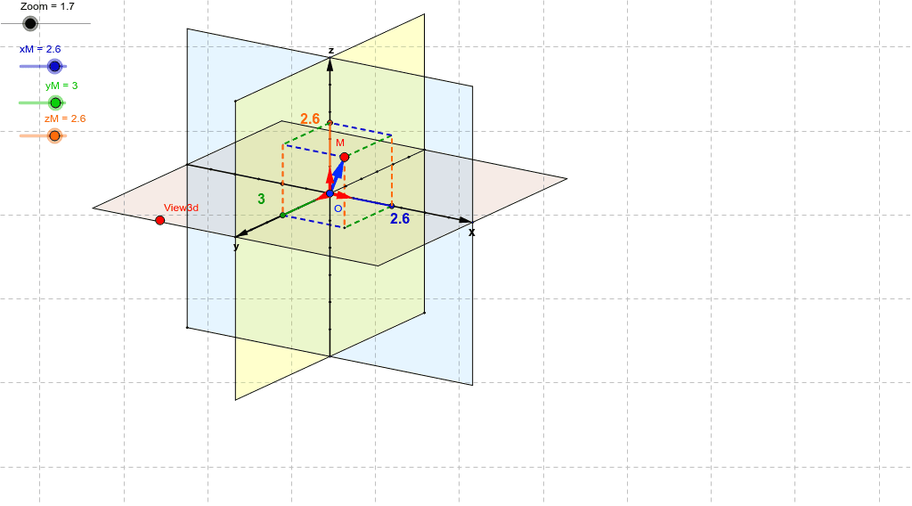
This example demonstrates the visualization of 3D vectors, covering core mathematical concepts like vector addition, reflection, and orthogonal lines. It utilizes commands such as Vector, OrthogonalLine, Translate, Midpoint, Line, Mirror, Segment, Intersect, and Polygon in GeoGebra for construction. Suitable for high school and above students learning 3D vectors and operations.
GeoGebra Commands & Parameters
Vector(B_1, X) → pVector(B_1, Z) → wOrthogonalLine(View3d, yAxis) → aOrthogonalLine(View3d, xAxis) → bVector(B_1, Y) → vTranslate(O, Vector[xM * p]) → ATranslate(A, Vector[yM * v]) → BTranslate(B, Vector[zM * w]) → MVector(O, M) → zMidpoint(O, M) → C1Translate(O, w) → GLine(O, G) → eTranslate(O, Vector[5 * w]) → HTranslate(O, Vector[-6 * w]) → IVector(I, H) → hTranslate(O, p) → KTranslate(O, Vector[6 * p]) → LMirror(L, O) → M_1Vector(M_1, L) → jTranslate(O, v) → NTranslate(O, Vector[6 * v]) → PMirror(P, O) → QSegment(A, B) → dLine(B, j) → nSegment(M, B) → qTranslate(O, Vector[zM * w]) → ESegment(E, M) → rVector(Q, P) → lLine(B, j) → fSegment(Q, P) → iVector(O, G) → p_1Vector(O, K) → sVector(O, N) → tMidpoint(O, K) → FMidpoint(O, N) → JMidpoint(G, O) → RMirror(O, K) → DMirror(K, D) → SMirror(D, S) → TMirror(S, T) → UMirror(K, O) → VMirror(O, V) → WMirror(V, W) → A1Mirror(W, A1) → B1Mirror(A1, B1) → D1Mirror(O, N) → E1Mirror(N, E1) → F1Mirror(E1, F1) → G1Mirror(G1, F1) → H1Mirror(F1, G1) → I1Mirror(N, O) → J1Mirror(O, J1) → K1Mirror(J1, K1) → L1Mirror(K1, L1) → M1Mirror(L1, M1) → N1Mirror(O, G) → O1Mirror(G, O1) → P1Mirror(O1, P1) → Q1Mirror(G, O) → R1Mirror(O, R1) → S1Mirror(R1, S1) → U1Mirror(S1, U1) → V1Mirror(U1, V1) → W1Translate(N, s) → Z1Line(L, l) → mLine(P, j) → a1Line(M_1, l) → b1Line(Q, j) → c1Intersect(b1, c1) → A2Intersect(m, c1) → B2Intersect(a1, m) → C2Intersect(a1, b1) → D2Polygon(A2, B2, C2, D2) → poly1, a2, b2, c2, d2Line(H, j) → d1Line(L, h) → e1Line(M_1, h) → f1Line(I, d1) → g1Intersect(d1, f1) → E2Intersect(e1, d1) → F2Intersect(g1, e1) → G2Intersect(g1, f1) → H2Polygon(E2, F2, G2, H2) → poly2, e2, f2, g2, h2Line(H, l) → h1Line(Q, h) → i1Line(P, h) → j1Line(I, l) → k1Intersect(h1, i1) → I2Intersect(j1, h1) → J2Intersect(k1, j1) → K2Intersect(i1, k1) → L2Polygon(I2, J2, K2, L2) → poly3, i2, j2, k2, l2Line(B, j) → l1Segment(O, P) → m1Intersect(l1, m1) → M2Segment(M2, B) → n1Segment(O, M2) → b_1Segment(O, A) → a_1Segment(A, C) → c_1Segment(C, M) → d_1Segment(M, A_1) → e_1Segment(O, E) → f_1Segment(C, E) → g_1Segment(E, A_1) → h_1Segment(A_1, M2) → i_1Segment(A, C) → j_1
AI Drawing Prompt Reference
Create a 3D vector visualization, including vectors p, w, and v, and their linear combinations forming point M, as well as the mirror image of vector w through the origin O. Start by drawing vectors p and w, then draw vector v, and construct point M using vectors p and w. Next, draw line e through origin O and vector w, then construct the mirror image of vector w, and finally draw vectors p, v, and their linear combinations forming point M, and connect related points to form segments and lines.
The prompt above was compiled from the original drawing commands and is for reference only.