
3D Circular Wave Demonstration
Loading the math board and drawing, please wait…
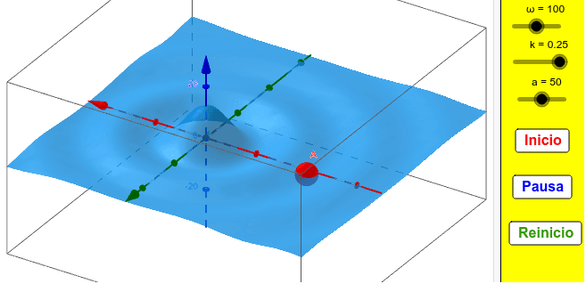
This example demonstrates the dynamic behavior of circular waves in 3D space. It involves core mathematical concepts such as functions, trigonometry, complex numbers, linear regression, and statistical characteristics. Key GeoGebra commands used in construction include angular frequency ω, wave number k, time t, amplitude a, frequency f, control buttons, and parameters like λ (wavelength) and A (phase). Suitable for high school and advanced mathematics education to visualize wave equations and parameter effects.
GeoGebra Commands & Parameters
Numeric ω(100.0)Numeric k(0.25)t:0a:50f(x, y) = (a / sqrt(x^(2) + y^(2)) * sin((k * sqrt(x^(2) + y^(2))) - (ω * t)))Line b(1.0, 0.0, 0.0)Line c(0.0, 1.0, 0.0)Line d(1.0, 0.0, 0.0)Line e(0.0, 1.0, 0.0)Line f_2(1.0, 0.0, 0.0)Line h(1.0, 0.0, 0.0)Line i(0.0, 1.0, 0.0)Line j(1.0, 0.0, 0.0)Line l(0.0, 1.0, 0.0)g(z) = sin((ω * t))(2 * π / k)(-40, 0, (a * sin((ω * t) + ((2 * π) * λ / 40)) / 20))