
刚体旋转
几何画板及绘图内容加载中,请稍等……
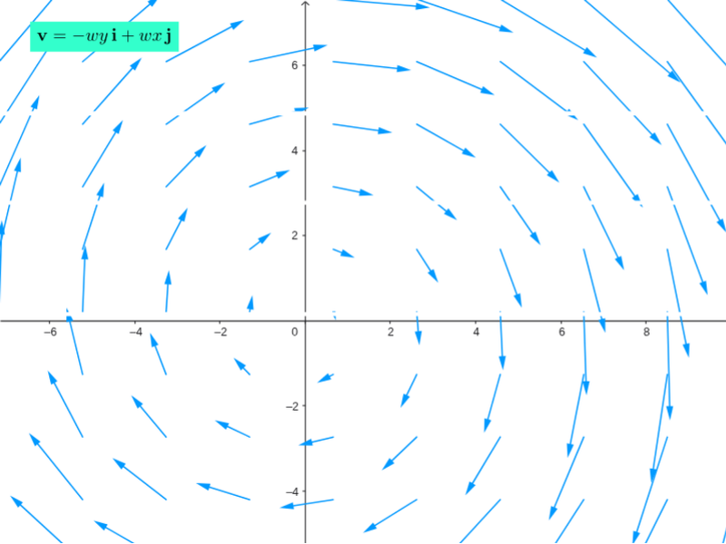
该范例演示了刚体旋转的几何现象。核心数学概念包括旋转矩阵和向量。通过使用GeoGebra命令如Sequence、Circle、Line等,可以动态展示刚体旋转过程中的几何变换。适合高中及以上学生学习几何变换和向量知识。
GeoGebra 命令及参数
Sequence(Sequence[Vector[(j, k), (j + (scale * F_1(j, k)), k + (scale * F_2(j, k)))], j, xmin, xmax, xstep], k, ymin, ymax, ystep) → vFieldSequence(((x(Element[inicialPts, i]) * cos((w * time))) - (y(Element[inicialPts, i]) * sin((w * time))), (x(Element[inicialPts, i]) * sin((w * time))) + (y(Element[inicialPts, i]) * cos((w * time)))), i, 1, 8) → particlesListSequence(CurveCartesian[(x(Element[inicialPts, i]) * cos((w * t))) - (y(Element[inicialPts, i]) * sin((w * t))), (x(Element[inicialPts, i]) * sin((w * t))) + (y(Element[inicialPts, i]) * cos((w * t))), t, 0, time], i, 1, 8) → pathlinesListSequence(Vector[Element[particlesList, i], (x(Element[particlesList, i]) + (scale * F_1(x(Element[particlesList, i]), y(Element[particlesList, i]))), y(Element[particlesList, i]) + (scale * F_2(x(Element[particlesList, i]), y(Element[particlesList, i]))))], i, 1, 8) → vectorParticlesSequence(Segment[Rotate[curlPt - (0.6, 0), k + curlAngle, curlPt], Rotate[curlPt + (0.6, 0), k + curlAngle, curlPt]], k, 0, 2.0944, 1.0472) → spokesCircle(divPt, 0.6) → divGlowCircleLine(I, xAxis) → fLine(J, xAxis) → gLine(K, xAxis) → h